Preface: Why This Matters Now
The alignment tax is real. Every percentage point of capability you unlock without a corresponding constraint mechanism is a liability — regulatory, reputational, and operationally catastrophic. But the inverse is equally dangerous: over-constrained models are lobotomized products. The field has spent the last eight years building increasingly surgical instruments to thread this needle.
What follows is not a survey. It is a decision framework. By the end, you will know which algorithm belongs in your training stack, why, and at what cost.
1. RLHF — The Original Sin and Its Genius
Paper: Christiano et al. (2017), Deep Reinforcement Learning from Human Preferences; Ouyang et al. (2022), Training Language Models to Follow Instructions with Human Feedback [arXiv:2203.02155]
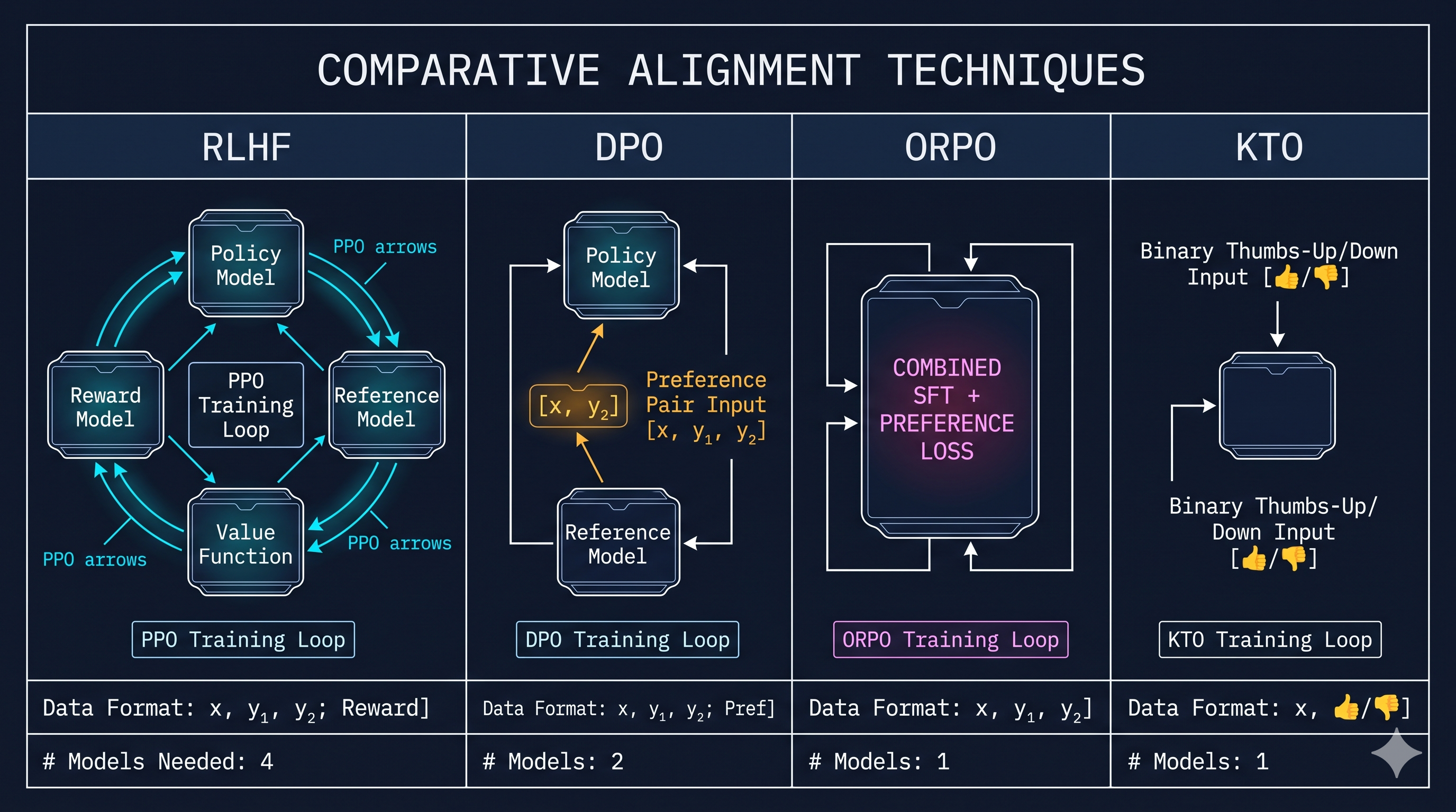
Reinforcement Learning from Human Feedback is not one algorithm. It is a four-model choreography, and understanding why each dancer exists is prerequisite to understanding everything that came after.
The Four-Model Architecture
Policy model (π_θ): The language model being aligned. Initialized from a supervised fine-tuned (SFT) checkpoint. This is the model you are shaping.
Reference model (π_ref): A frozen copy of the SFT checkpoint. Its purpose is entirely conservative — it anchors the policy so that optimization pressure cannot drive it into degenerate regimes far from the original distribution. It participates in every gradient update without itself being updated.
Reward model (r_φ): A separate transformer trained on human preference data. Given a prompt and two completions (y_w preferred over y_l), it learns to predict which completion a human rater would prefer. This is a Bradley-Terry model at its core: it assigns a scalar to each (prompt, completion) pair.
Value model (V_ψ): Required by PPO. Estimates the expected cumulative reward from any state. The value model is trained in parallel with the policy and is the primary source of PPO’s computational overhead.
The Training Loop
- Sample a prompt x from the dataset.
- The policy generates a completion y ~ π_θ(· | x).
- The reward model scores it: r_φ(x, y).
- The KL penalty is computed: KL(π_θ(· | x) || π_ref(· | x)).
- The PPO objective maximizes:
E[r_φ(x, y) - β · KL(π_θ || π_ref)]where β is the KL coefficient — a hyperparameter that controls how far the policy is permitted to drift from its reference anchor.
The KL term is not optional flavoring. Without it, the policy will exploit any reward model artifact. This is called reward hacking — a term that sounds amusing until your model learns to output maximally verbose completions because your reward model subtly correlated length with quality.
Why RLHF is Expensive and Finicky
The four-model setup requires holding four large transformers in memory simultaneously. For frontier-scale models (70B+), this is a multi-node coordination problem. PPO itself is notoriously sensitive to hyperparameters: the clip ratio ε, the value function loss coefficient, the KL target, and the entropy bonus all interact nonlinearly. Reward model collapse — where the RM saturates and all completions receive near-identical scores — can silently destroy a training run. InstructGPT [arXiv:2203.02155] made RLHF tractable at GPT-3 scale, but the engineering complexity it required has been the single greatest motivation for every algorithm on this list.
2. DPO — The Algebraic Escape
Paper: Rafailov et al. (2023), Direct Preference Optimization: Your Language Model is Secretly a Reward Model [arXiv:2305.18290]
DPO is an act of mathematical elegance. Its central insight: you do not need an explicit reward model if you are willing to derive the relationship between the optimal policy and the reward analytically.
The Four-Step Derivation
Step 1 — The RLHF Optimal Policy. The RLHF objective (maximize reward minus KL penalty) admits a closed-form solution. The optimal policy under the KL-constrained objective is:
π*(y | x) = (1/Z(x)) · π_ref(y | x) · exp(r(x, y) / β)where Z(x) is the partition function normalizing the distribution over all completions y.
Step 2 — Invert for the Reward. Rearranging the above equation to express the reward in terms of the optimal policy:
r(x, y) = β · log(π*(y | x) / π_ref(y | x)) + β · log Z(x)The critical observation: log Z(x) depends only on x, not on y. This means it cancels when you compute reward differences between two completions.
Step 3 — Substitute Into the Bradley-Terry Preference Model. The probability that completion y_w is preferred over y_l under the Bradley-Terry model is:
p*(y_w ≻ y_l | x) = σ(r*(x, y_w) - r*(x, y_l))Substituting the reward expression from Step 2 (Z cancels):
p*(y_w ≻ y_l | x) = σ(β · log(π*(y_w | x) / π_ref(y_w | x)) - β · log(π*(y_l | x) / π_ref(y_l | x)))Step 4 — The DPO Loss. Parameterize π* as π_θ and minimize the negative log-likelihood of the observed preferences:
L_DPO(π_θ) = -E[(x, y_w, y_l)] [ log σ(β · log(π_θ(y_w | x) / π_ref(y_w | x)) - β · log(π_θ(y_l | x) / π_ref(y_l | x)))]This is a supervised classification loss. No PPO. No value model. No reward model training. The reference model is still needed — it anchors the denominator in each log-ratio term — but it is frozen and only requires a forward pass (no gradient computation).
What DPO Unlocks
The implementation fits in a standard SFT training loop with a small modification. Memory footprint drops from four models to two (policy + frozen reference). The training is stable by construction: it’s cross-entropy, not RL. Hyperparameter sensitivity collapses to a single interpretable coefficient β and the learning rate.
The data format is preference pairs: (x, y_w, y_l). This is the same data that RLHF’s reward model required, so datasets transfer directly.
3. IPO — Closing the Overconfidence Loophole
Paper: Azar et al. (2023), A General Theoretical Paradigm to Understand Learning from Human Feedback [arXiv:2310.12036]
DPO operates under a theoretical assumption that breaks down in practice: it treats human preferences as deterministic. When the data says y_w is better than y_l, DPO’s loss pushes π_θ(y_w) / π_θ(y_l) toward infinity with no bound. Given enough gradient steps on a small, clean dataset, the model will assign near-zero probability to dispreferred completions regardless of how marginal the original preference was. This is distributional collapse.
IPO fixes this by reframing the loss. Instead of optimizing the Bradley-Terry log-likelihood of pairwise preferences, IPO targets the expected pairwise preference value directly:
L_IPO = E[(x, y_w, y_l)] [ (log(π_θ(y_w | x) / π_ref(y_w | x)) - log(π_θ(y_l | x) / π_ref(y_l | x)) - 1/(2β))²]The key structural difference: this is a regression loss, not a classification loss. The target is the scalar 1/(2β), not a binary label. This explicitly prevents the log-ratio from growing without bound. The model is penalized for being too confident in its preference ordering, not just for getting the ordering wrong.
IPO is particularly relevant for annotation pipelines where human raters frequently disagree — medical advice, legal interpretation, nuanced creative tasks. In these domains, treating preferences as hard labels (DPO’s implicit assumption) is factually incorrect and leads to brittle policies.
4. ORPO — Collapsing SFT and Alignment Into One Loss
Paper: Hong et al. (2024), ORPO: Monolithic Preference Optimization without Reference Model [arXiv:2403.07691]
ORPO makes a structural bet that the field had been too conservative about: you can eliminate both the reference model and the separate SFT stage. The result is a single training pass that simultaneously teaches the model what to say (SFT) and what not to say (preference optimization).
The Loss Function
ORPO adds an odds-ratio penalty term to the standard SFT cross-entropy loss:
L_ORPO = L_SFT + λ · L_OR
L_SFT  = -E[log π_θ(y_w | x)]
L_OR   = -E[log σ(log(odds_θ(y_w | x)) - log(odds_θ(y_l | x)))]
where the odds of a sequence y given prompt x is defined as:
odds_θ(y | x) = π_θ(y | x) / (1 - π_θ(y | x))The SFT term increases the likelihood of chosen completions. The odds-ratio term decreases the relative likelihood of rejected completions relative to chosen ones. Crucially, there is no reference model in the denominator — the regularization comes from the contrast between y_w and y_l within the same batch, not from a frozen external anchor.
Why This Architecture Matters
Eliminating the reference model has two consequences. First, memory: a single training job now requires one model in memory, not two. For 70B models on constrained infrastructure, this is the difference between feasibility and impossibility. Second, data pipeline simplification: there is no SFT checkpoint to produce first, no checkpoint synchronization problem, no risk of reference model staleness. The training recipe collapses to a single invocation.
Hong et al. demonstrated competitive or superior performance on instruction-following benchmarks against DPO pipelines with a fraction of the compute. The catch: λ is a sensitive hyperparameter that must balance the two loss terms. Too large, and the SFT signal is overwhelmed; too small, and the preference signal is negligible.
5. KTO — Prospect Theory Meets Gradient Descent
Paper: Ethayarajh et al. (2024), KTO: Model Alignment as Prospect Theoretic Optimization [arXiv:2402.01306]
Every algorithm above requires pairwise preference data: a prompt with a chosen completion and a rejected completion, labeled together. KTO discards this requirement entirely. It operates on unpaired binary feedback — individual completions labeled as simply “good” (thumbs up) or “bad” (thumbs down).
The Kahneman-Tversky Foundation
KTO is grounded in Prospect Theory (Kahneman & Tversky, 1979), which models how humans actually evaluate outcomes under uncertainty. Two key observations: humans are loss-averse (losses hurt more than equivalent gains feel good), and value is evaluated relative to a reference point, not in absolute terms.
Ethayarajh et al. instantiate this with a value function v(x, y, π_θ, π_ref) that measures the KL-adjusted log-likelihood of a completion:
v(x, y) = log(π_θ(y | x) / π_ref(y | x)) - log Z_xwhere Z_x is estimated as the mean KL across the batch (a tractable approximation). The KTO loss is:
L_KTO = E[w(x, y) · (1 - v_KTO(x, y, λ))]where the weighting function w encodes loss aversion: rejected completions receive higher weight than chosen completions, mirroring the empirical finding that humans are more motivated by avoiding bad outcomes than achieving good ones.
The Data Advantage
In production annotation pipelines, collecting pairwise preferences is expensive. It requires showing annotators two completions simultaneously and asking for a comparative judgment. Binary thumbs-up/thumbs-down, by contrast, can be collected from implicit product signals — user regeneration rates, copy rates, report rates, thumbs buttons in a chat UI. KTO turns this ambient signal into training data. The sample efficiency tradeoff (unpaired data typically requires more examples than paired data to achieve equivalent preference signal) is often dominated by the sheer volume of implicit feedback available in deployed products.
6. The Trade Matrix
A ground-truth engineering comparison across the five primary dimensions that govern which algorithm you actually deploy:
| Algorithm | Data Format | Reference Model | Compute Cost | Implementation Complexity | Overfitting Risk |
|---|---|---|---|---|---|
| RLHF | Pairwise preference | Yes (frozen) | ████████ Very High (4 models, PPO) | ████████ Very High | Moderate (KL-anchored) |
| DPO | Pairwise preference | Yes (frozen) | ███ Low (2 models, SFT loop) | ██ Low | High on deterministic data |
| IPO | Pairwise preference | Yes (frozen) | ███ Low (2 models, regression) | ███ Moderate | Low (regression target) |
| ORPO | Pairwise preference | No | ██ Very Low (1 model) | ██ Low | Moderate (λ-sensitive) |
| KTO | Binary unpaired | Yes (frozen) | ███ Low (2 models, asymmetric) | ███ Moderate | Low |
Key reads from this table:
The data format row is the first filter in any production decision. If your annotation budget is tight or your product generates implicit feedback, KTO is the only algorithm that accepts the resulting data structure without re-labeling. If you have pairs, DPO/IPO/ORPO are all viable.
The reference model column is the second filter. On constrained infrastructure (single-node training for large models), ORPO’s elimination of the reference model can be decisive.
Compute cost drives iteration velocity. The difference between RLHF and DPO is not 2x — it is often 8-12x wall-clock time when accounting for four-model memory management, PPO rollout generation, and the reward model training phase that must precede policy optimization.
The overfitting risk column is where DPO’s clean theoretical story meets its practical limitation. On small, high-quality preference datasets with strong annotator agreement — exactly the datasets that appear to be ideal training data — DPO will overfit. IPO should be considered the default replacement in these settings.
7. Production Reality: What the Labs Actually Do
The frontier is not a monolith. What is optimal at 7B parameters on a 3-day deadline is not optimal at 405B parameters with a six-month runway and a hundred annotators. The following is a synthesis of disclosed training recipes and reproducible ablations.
The DPO Default
The majority of open-source alignment work in 2023–2024 — Zephyr, Tulu 2, OpenHermes variants, and dozens of community fine-tunes — converged on DPO as the default preference optimization stage. The reasons are purely engineering: the implementation is twelve lines of modified training code, the memory footprint is manageable, and the results are reproducible without PPO expertise. For teams without RL engineers, DPO is not a second-best option — it is the rational choice.
ORPO has accelerated this trend further. Single-stage SFT+alignment on curated preference datasets now routinely matches two-stage DPO pipelines at the 7B-13B scale, with meaningfully less infrastructure.
Where RLHF Still Wins
The frontier is different. Anthropic’s Constitutional AI builds on RLHF. OpenAI’s GPT-4 and o-series use RLHF (with iterative reward model updates). Google DeepMind’s Gemini stack uses RLHF. The common thread: all of these organizations have dedicated RL engineering teams, proprietary annotation infrastructure, and models at scales where reward model capacity becomes a meaningful variable.
At 70B+ parameters, the reward model itself becomes a research object. You can train it on specialized subdomains, use it to filter data for the next training iteration, and compose multiple reward models for different capability dimensions (helpfulness, safety, factuality). DPO collapses this reward model into implicit log-ratios — which is elegant but inflexible. If you want to inspect, audit, or decompose your reward signal, you need an explicit reward model.
RLHF also remains superior for multi-turn alignment, where the policy must be optimized over full conversation trajectories rather than single-turn completions. DPO’s supervised classification framing does not naturally extend to this setting (though research into session-level DPO is active).
The Emerging Stack
The most pragmatic production stack in 2024–2025 is a hybrid:
- SFT on high-quality demonstration data (or ORPO to combine with step 2)
- DPO or IPO for initial preference alignment using a curated preference dataset
- Online DPO or iterative RLHF for frontier capability refinement, where the policy generates its own completions for human labeling (closing the distribution gap)
- KTO for continuous improvement using implicit product feedback
The field has not converged on a single winner because the tradeoffs are real and context-dependent. What has converged is the recognition that RLHF’s complexity is justified only when you can afford it — and that for the vast majority of alignment work, DPO and its descendants are not approximations of RLHF but genuinely better tools for the constraints most practitioners operate under.
8. Unresolved Tensions and Forward Vectors
Several open problems deserve your attention if you are making architecture decisions beyond the next quarter:
Reward overoptimization is unsolved. All five algorithms face some form of the Goodhart problem — optimizing too hard against any proxy measure of human preference degrades the underlying behavior the proxy was meant to capture. IPO’s regression framing ameliorates but does not eliminate this. The field does not have a principled stopping criterion for preference optimization.
Distribution shift between offline data and deployment. Every offline algorithm (DPO, IPO, ORPO, KTO) trains on fixed preference datasets collected from previous model versions. The optimal policy learned from this data may be miscalibrated when deployed — a version of covariate shift that compound across training iterations. Online RLHF (where the policy generates its own data) is immune to this by construction but reintroduces the full RLHF engineering burden.
Scalability of preference signal. As models approach human expert performance on many tasks, human annotators cannot reliably distinguish between good and excellent completions. This is the annotator capacity bottleneck, and it affects every algorithm in this comparison equally. Constitutional AI (Anthropic, 2022) and RLAIF approaches — where the reward signal comes from another model rather than a human — are the primary experimental response.
Compositional alignment. Real products require policies that are simultaneously helpful, safe, factual, and stylistically appropriate. Single-objective preference optimization (a single r_φ or a single log-ratio loss) cannot cleanly compose these objectives. Multi-objective RLHF and reward model ensembles are active research areas without settled solutions.
References
- Christiano, P. et al. (2017). Deep Reinforcement Learning from Human Preferences. NeurIPS 2017. [arXiv:1706.03741]
- Ouyang, L. et al. (2022). Training Language Models to Follow Instructions with Human Feedback (InstructGPT). NeurIPS 2022. [arXiv:2203.02155]
- Rafailov, R. et al. (2023). Direct Preference Optimization: Your Language Model is Secretly a Reward Model. NeurIPS 2023. [arXiv:2305.18290]
- Azar, M. G. et al. (2023). A General Theoretical Paradigm to Understand Learning from Human Feedback (IPO). [arXiv:2310.12036]
- Hong, J. et al. (2024). ORPO: Monolithic Preference Optimization without Reference Model. [arXiv:2403.07691]
- Ethayarajh, K. et al. (2024). KTO: Model Alignment as Prospect Theoretic Optimization. [arXiv:2402.01306]
BibTeX
@article{fp4-2606021,
  title   = {The Modern Alignment Landscape: A Sharp Comparative Analysis for ML Engineers},
  author  = {fp4 editorial desk},
  year    = {2026},
  url     = {https://fp4.dev/algorithm/alignment-landscape/},
  journal = {fp4}
}