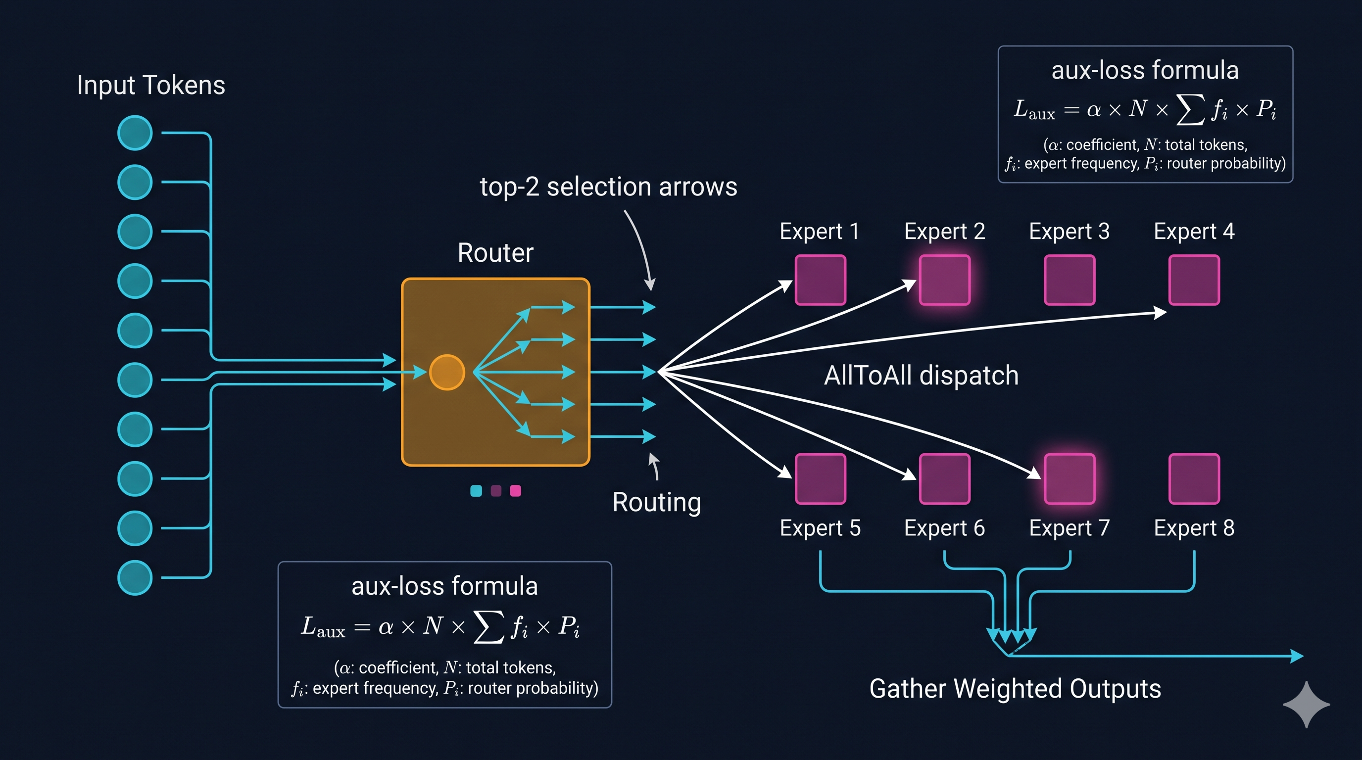
“The best model is the one that spends its FLOPs where the problem actually lives — not uniformly across a monolith.”
Preface: Why MoE Is Not Just a Trick
Most ML practitioners first encounter Mixture-of-Experts as a clever parameter efficiency story. That framing is dangerously incomplete. MoE is simultaneously a computational routing architecture, a distributed systems contract, a gradient flow engineering challenge, and a production serving puzzle — all wrapped into a single abstraction. Getting any one of these wrong cascades catastrophically into the others.
This article dissects each layer with the precision a systems engineer needs: from the mathematical gating formulation to AllToAll network topology, from auxiliary loss design to the “fat node” serving pattern that sidesteps inter-GPU communication entirely.
1. The Parameter-Compute Decoupling Insight
The foundational MoE observation — articulated rigorously by Shazeer et al. (2017) and operationalized at scale by the Switch Transformer (Fedus et al., 2022 [2101.03961]) — is deceptively elegant:
Total model parameters can grow without per-token compute growing.
In a standard dense transformer, doubling parameters doubles FLOPs per token. MoE breaks this coupling. Consider a transformer where each FFN sub-layer is replaced by E independent expert networks. If each token routes to only k of those E experts, the per-token FLOPs scale with k, not E. You can grow E — and thus total parameter count — while holding k (and therefore compute) fixed.
Formally, let each expert i be a function f_i : ℝ^d → ℝ^d. For a given input token x, the MoE layer output is:
MoE(x) = Σ_{i ∈ TopK(x)} g_i(x) · f_i(x)where g_i(x) are scalar gate weights (defined below) and the sum runs over only the k selected experts. If each expert is an FFN of dimension d_ff, per-token FLOPs are O(k · d · d_ff) — independent of total expert count E.
What does this buy you in practice?
Mixtral 8×7B [2401.04088] has ~46.7B total parameters but activates roughly 12.9B per token (2-of-8 experts). It matches or exceeds LLaMA-2 70B on most benchmarks at approximately one-third the inference compute. DeepSeek-V3 [2412.19437] scales this further: 671B total parameters, 37B active per token (8-of-256 fine-grained experts, plus shared experts). The ratio of total-to-active parameters is 18:1 — an extraordinary leverage ratio that dense models can never achieve.
The intuition is that a model learns to partition the semantic space across experts. Syntax-heavy tokens route to different experts than arithmetic tokens, which route differently from medical vocabulary. Specialization emerges from routing pressure, not explicit design.
2. The Router: Gating Mathematics and the Differentiability Problem
2.1 Router Architecture
The router is architecturally simple: a linear projection from the token’s hidden state x ∈ ℝ^d into a logit vector over E experts, followed by a selection and normalization step.
Router logits:    h(x) = W_r · x        where W_r ∈ ℝ^{E×d}
Gate scores:      s(x) = Softmax(h(x))  ∈ ℝ^E
Top-k selection:  TopK(s, k) → indices I ⊆ {1,...,E}, |I| = k
Renormalized gates: g_i(x) = s_i(x) / Σ_{j ∈ I} s_j(x)   for i ∈ I                    g_i(x) = 0                               otherwise
The renormalization step (dividing by the sum of selected scores) is critical. It ensures the gate weights for the chosen experts sum to 1, preserving the output magnitude regardless of how confident or diffuse the routing decision is.
Typical values of k:
| Model | E (experts) | k (active) | Active ratio |
|---|---|---|---|
| Switch Transformer | 128–2048 | 1 | <1% |
| Mixtral 8×7B | 8 | 2 | 25% |
| Qwen-MoE | 64 | 4 | 6.25% |
| DeepSeek-V3 | 256 | 8 | 3.125% |
Switch Transformer used k=1 (a single expert per token) — maximally sparse, minimal compute, but high variance. Mixtral’s k=2 provides redundancy that improves quality with modest cost. DeepSeek-V3’s k=8-of-256 achieves ultra-fine-grained specialization: 256 small experts each covering a narrow semantic niche, with 8 selected per token — a design that maximizes expert utilization diversity.
2.2 The Differentiability Problem and the Soft-Gate Trick
Here lies a subtle but critical issue: top-k selection is not differentiable.
The indicator function that decides whether expert i is selected is a step function with zero gradient almost everywhere. Naive backpropagation through a hard top-k gate gives no learning signal to the router weights W_r for experts that were not selected — but those are exactly the experts we need the router to learn to route away from.
The resolution is the soft gate weight trick: gradients flow not through the selection decision itself, but through the values of the soft scores for the selected experts.
Consider the forward pass: we compute full softmax probabilities s(x) over all E experts, perform hard top-k selection to identify I, then multiply expert outputs by g_i(x) = s_i(x) / normalization for i ∈ I. During backpropagation, ∂Loss/∂g_i flows through the renormalized gate value g_i, back through the softmax, and into W_r.
∂Loss/∂W_r = Σ_{i ∈ I} (∂Loss/∂g_i) · (∂g_i/∂s_i) · (∂s_i/∂h_i) · x^TThe Jacobian ∂g_i/∂s_i from the renormalized softmax is well-defined and non-zero. So even though the discrete selection doesn’t differentiate, the magnitude of soft scores for selected experts does — and this is sufficient to train the router to make good routing decisions. The router learns: “increase the logit for expert i on tokens like x because expert i gave a useful output there.”
This gradient signal is real but imperfect. Experts not selected receive zero gradient from the gating path for that token. This is why load balancing losses (Section 3) are essential — they provide a gradient signal that prevents the router from collapsing to a degenerate solution.
3. Load Balancing: Preventing Expert Collapse
3.1 The Expert Collapse Problem
Left to its own devices during training, MoE routing tends toward catastrophic expert collapse: one or two experts receive the vast majority of tokens, while others receive almost nothing and consequently fail to develop useful representations. The winning experts receive more gradient signal, improve faster, attract more routing, and the feedback loop completes. The result is an expensive dense model masquerading as an MoE.
This is not a theoretical concern. Early MoE experiments observed expert utilization distributions where the top expert handled >60% of tokens in a 64-expert model. The 63 neglected experts wasted ~97% of parameter capacity.
3.2 The Switch Transformer Auxiliary Loss
Fedus et al. [2101.03961] introduced the canonical load-balancing auxiliary loss, added to the training objective to encourage uniform token distribution across experts.
Let T be the total number of tokens in a batch, E the number of experts. Define:
f_i = (1/T) · Σ_{x in batch} 𝟙[token x routed to expert i]    (fraction of tokens → expert i)
P_i = (1/T) · Σ_{x in batch} s_i(x)                           (mean routing probability for expert i)
The auxiliary loss is:
L_aux = α · E · Σ_{i=1}^{E} f_i · P_iwhere α is a hyperparameter (typically 0.01–0.1). The factor E normalizes so that perfect balance (f_i = 1/E for all i) gives L_aux = α regardless of E.
Why does this work? f_i measures actual token routing (discrete, not differentiable). P_i measures soft routing probability (differentiable). Their product creates a differentiable signal: if expert i is overloaded (f_i large), the loss penalizes high P_i, pushing the router to assign lower probability to expert i in future steps. The product makes the gradient flow through the soft probabilities, allowing the optimizer to redistribute routing pressure.
The hyperparameter α requires careful tuning. Too small: collapse persists. Too large: the balancing loss dominates, routing becomes quasi-uniform, and specialization collapses — different failure mode, same symptom (degraded model quality).
3.3 DeepSeek-V3’s Auxiliary-Loss-Free Balancing
DeepSeek-V3 [2412.19437] introduces a more surgical approach: auxiliary-loss-free load balancing via dynamic bias adjustment. The insight is that the auxiliary loss perturbs the primary training objective — every gradient step is a compromise between “learn to route well for task performance” and “maintain balance.” At scale, this tension accumulates into measurable quality degradation.
DeepSeek-V3’s solution: maintain a per-expert bias term b_i that is updated separately from the main model weights, using a simple heuristic rule rather than gradient descent:
Routing logit (modified): h_i(x) + b_iSelection: TopK over modified logits (for routing decision only)Gate weights: Computed from original h_i(x) without bias (for output computation)The bias b_i is updated after each training step:
- If expert i was overloaded in the last step: b_i ← b_i − γ
- If expert i was underloaded: b_i ← b_i + γ
where γ is a small step size. This decouples balancing pressure from the primary gradient flow. The main model parameters train purely on task loss; balance is maintained through the external bias controller. The result: better model quality at the same level of load balance. DeepSeek-V3 reports this approach achieves near-perfect balance without the auxiliary loss compromising primary task gradients.
4. Communication Topology: AllToAll Is the New AllReduce
4.1 Expert Parallelism and the Communication Contract
In a distributed training or inference setup with Expert Parallelism (EP), each GPU (or group of GPUs) hosts a subset of experts. Tokens arrive at all GPUs after the attention layer, but each token must be sent to whichever GPU hosts its designated expert(s). This creates a fundamentally different communication pattern than standard tensor or pipeline parallelism.
The communication pattern is AllToAll: every GPU sends a different subset of tokens to every other GPU, and receives a different subset back. After expert computation, the gathered results must be assembled and returned to the originating GPUs.
Forward pass:[Tokens on GPU 0] --dispatch--> [Experts on GPU 0, 1, 2, ..., N-1] ↓ (expert computation)[Results from GPU 0, 1, 2, ..., N-1] --gather--> [Assembled output on GPU 0]Two AllToAll operations per MoE layer (one to dispatch tokens, one to gather results). In contrast, tensor parallelism uses AllReduce — which, while expensive, has highly optimized collective implementations (NCCL ring-allreduce). AllToAll at large EP degrees is harder to optimize and more sensitive to network topology.
4.2 Quantifying the AllToAll Bottleneck
Consider a concrete example: 256 experts distributed across 32 GPUs (8 experts/GPU), serving a batch of T=1024 tokens, hidden dimension d=7168 (DeepSeek-V3 scale), with k=8 active experts per token. Assuming bfloat16 (2 bytes/element):
Tokens dispatched per token: k = 8 expertsEach token representation: d = 7168 elements × 2 bytes = 14,336 bytes ≈ 14 KB
Total dispatch volume per step:  T × k × d × 2 bytes = 1024 × 8 × 7168 × 2 = ~117 MB
With node-limited routing (max 4 nodes), cross-node traffic reduced to:  ~29 MB per AllToAll phase
With InfiniBand HDR at 200 Gb/s effective bandwidth per link, 117 MB takes ~4.7 ms per AllToAll. Two AllToAll operations per MoE layer, with 61 MoE layers in DeepSeek-V3: ~573 ms of pure AllToAll latency in the critical path per forward pass at batch size 1024 — before any computation. Expert parallel efficiency drops precipitously as EP degree grows, because AllToAll volume grows with the number of participating GPUs.
This is why DeepSeek-V3 introduced node-limited routing: each token’s 8 experts must span at most 4 nodes, bounding cross-node AllToAll traffic. Intra-node NVLink AllToAll is ~10× faster than inter-node InfiniBand, so constraining routing to minimize inter-node hops is a major throughput win. The router learns routing patterns that satisfy this constraint, and training enforces it via a hard routing constraint added during the policy.
5. Serving Challenges: Batching, Locality, and the Fat Node Pattern
5.1 Expert-Level Batching and the Padding Trap
Dense model inference benefits from batching: more tokens per step improves GPU utilization by amortizing compute across the matmul. MoE serving has a structural challenge: expert load is non-uniform across a batch.
If batch size is B and k=2, the average load per expert is 2B/E tokens. But variance is high — some experts will receive significantly more tokens than average, others fewer. The forward pass cannot complete until the most-loaded expert finishes. Underloaded experts sit idle, wasting compute. This is the serving analog of the expert collapse problem during training.
Practical mitigations:
Expert choice routing (used in some inference frameworks): Rather than each token choosing its top-k experts, each expert chooses its top-m tokens from the batch. This guarantees exactly m tokens per expert, eliminating load imbalance. The tradeoff: some tokens may not reach all their desired experts (or may be dropped). For serving where throughput matters more than per-token coverage, this is often acceptable.
Token padding: Pad each expert’s input batch to a fixed capacity C. Allows static shape computation, critical for CUDA kernel fusion and XLA compilation. The padding wastes FLOPs but enables significantly faster kernels. Switch Transformer used capacity factor C = k·T/E·factor where factor ∈ [1.0, 2.0].
5.2 Expert Cache Locality
In systems where the full MoE is distributed across GPUs, each GPU holds a subset of expert weights. A request hitting expert i on GPU j requires j to have expert i’s weights resident in HBM. This is structurally guaranteed in expert parallelism, but creates cache locality challenges in speculative decoding and continuous batching scenarios.
Consider speculative decoding with a draft model: the draft model generates tokens speculatively, which the verifier (the large MoE) must evaluate. Token verification requires expert computation; different speculative tokens will route to different experts on different GPUs. The verification step may exhibit poor locality if speculative tokens are semantically diverse.
Expert weight offloading compounds this: on memory-constrained systems, experts not recently used may be offloaded to CPU DRAM or SSD. Expert selection for a new token triggers a weight prefetch with 10–100µs latency. Systems like LLM.int8() and llama.cpp implement expert offloading but must carefully prefetch based on routing predictions to hide this latency.
5.3 The Fat Node Pattern
The most elegant engineering solution to AllToAll overhead is to eliminate it entirely: the Fat Node pattern, where all experts for a given MoE layer reside on a single physical server.
A server with 8×H100 GPUs and NVLink Switch fabric achieves ~900 GB/s bidirectional NVLink bandwidth. Intra-server AllToAll at this bandwidth takes ~0.13 ms for the same 117 MB example above — 36× faster than InfiniBand. By constraining the MoE to one node per layer (or per MoE block), the expensive inter-node AllToAll disappears.
The constraint: server memory must hold all expert weights for the served layers. DeepSeek-V3’s fine-grained experts (each expert is deliberately smaller than in Mixtral) are designed to fit this pattern. With 256 experts of reduced parameter count per layer, total expert weight per layer can be arranged to fit within an 8-GPU fat node’s aggregate HBM (~640 GB at 80 GB/GPU). Pipeline parallelism then spans nodes across layers, not experts within layers.
6. DeepSeek-V3 Specifics: Fine-Grained Experts, Shared Experts, and Node-Limited Routing
DeepSeek-V3 [2412.19437] represents the current frontier of MoE system design. Its architecture departs from the Mixtral/Switch template in three critical dimensions:
6.1 Fine-Grained Experts
Where Mixtral uses 8 experts of size ~7B parameters each, DeepSeek-V3 uses 256 experts of much smaller individual size. The total parameter budget per MoE layer is similar, but the granularity of specialization is radically higher. Fine-grained experts allow the router to express nuanced token-to-expert affinity that coarse-grained designs cannot represent.
The router operates over 256 logits per token, applies temperature scaling for sharper distributions, and selects top-8. The resulting routing distribution is significantly more expressive: a token can simultaneously consult experts specializing in code syntax, mathematical reasoning, natural language coherence, and factual recall — all within a single MoE layer’s 8 activations.
6.2 Shared Experts
DeepSeek-V3 introduces shared experts: a small number of experts (2 in DeepSeek-V3) that receive every token, regardless of routing. Every token’s MoE output is:
Output(x) = Σ_{i ∈ TopK(x,8)} g_i(x)·f_i(x) + Σ_{j ∈ shared} f_j(x)The shared experts act as a universal base representation, capturing information that should be present regardless of token type. Specialized experts then add token-specific transformations on top. This hybrid design improves quality by ensuring that general linguistic processing is never accidentally routed away — a risk with pure top-k routing where some tokens might get routed to only highly specialized experts.
Shared experts also alleviate load balancing pressure: since shared experts receive all tokens, they don’t participate in the balancing problem. This lets the dynamic bias controller focus its balancing efforts on the 256 routable experts.
6.3 Node-Limited Routing Constraint
DeepSeek-V3 enforces a hard constraint during both training and inference: each token’s 8 selected experts must reside on at most 4 physical nodes. This is not a soft preference — it is enforced by the routing algorithm.
Implementation: the routing selects top-8 from the full 256 experts but applies a node-diversity constraint during beam selection. If preliminary top-8 would require 6 nodes, the algorithm substitutes lower-ranked experts from already-included nodes to reduce node count to ≤4.
The consequence on model quality: minimal, because 4 nodes × 64 experts/node = 256 experts are still accessible — the constraint only reduces the worst-case cross-node traffic without significantly constraining which semantic combinations are expressible. The consequence on communication cost: cross-node AllToAll volume is halved relative to unconstrained routing, directly improving throughput at scale.
7. Synthesis: The MoE Engineering Stack
Understanding MoE end-to-end means holding five simultaneous abstractions in mind:
┌─────────────────────────────────────────────────────────────┐│ MATHEMATICAL LAYER ││ Top-k gating with soft weight gradients ││ Auxiliary loss or bias-based balancing │├─────────────────────────────────────────────────────────────┤│ COMPUTE LAYER ││ k active experts × FFN FLOPs, fixed regardless of E ││ Expert specialization emerges from routing pressure │├─────────────────────────────────────────────────────────────┤│ MEMORY LAYER ││ Total params = E × expert_size (all must fit somewhere) ││ Active params = k × expert_size (must fit in HBM) │├─────────────────────────────────────────────────────────────┤│ COMMUNICATION LAYER ││ AllToAll dispatch + gather per MoE layer ││ Node-limited routing minimizes inter-node traffic │├─────────────────────────────────────────────────────────────┤│ SERVING LAYER ││ Expert-choice batching for load balance ││ Fat node pattern to eliminate cross-node AllToAll ││ Expert cache management for low-latency serving │└─────────────────────────────────────────────────────────────┘Each layer has its own failure modes and optimization levers. A model trained with perfect load balance can still underperform in serving if expert batching is naive. Perfect serving infrastructure is moot if the router collapses during training. The engineer who masters all five layers simultaneously builds systems that work — not just train.
References
- Shazeer, N., et al. (2017). Outrageously Large Neural Networks: The Sparsely-Gated Mixture-of-Experts Layer. ICLR 2017.
- Fedus, W., Zoph, B., & Shazeer, N. (2022). Switch Transformers: Scaling to Trillion Parameter Models with Simple and Efficient Sparsity. arXiv:2101.03961.
- Jiang, A., et al. (2024). Mixtral of Experts. arXiv:2401.04088.
- DeepSeek-AI. (2024). DeepSeek-V3 Technical Report. arXiv:2412.19437.
BibTeX
@article{fp4-2606018,
  title   = {Mixture-of-Experts Internals: A Systems Engineer's Field Manual},
  author  = {fp4 editorial desk},
  year    = {2026},
  url     = {https://fp4.dev/algorithm/moe-internals/},
  journal = {fp4}
}