Positional Encoding in Transformers: A First-Principles Engineering Treatise

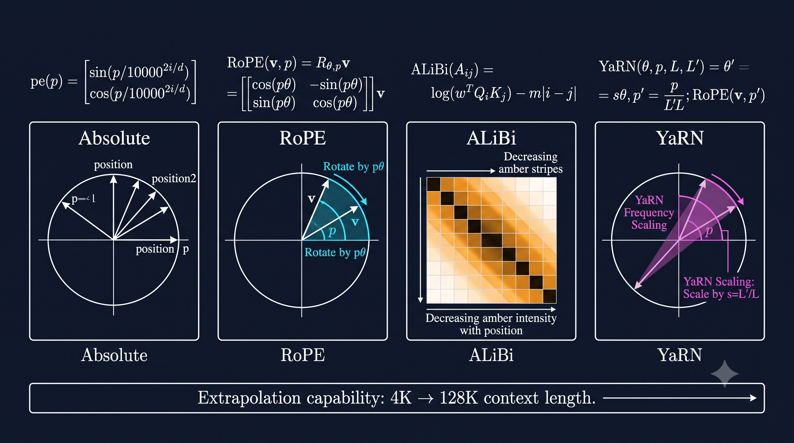
1. The Fundamental Problem: Attention Is Blind to Order

To understand why positional encoding exists, you must first internalize what self-attention actually computes — and what it deliberately does not.

Given a sequence of token embeddings $X = [x_1, x_2, \ldots, x_n] \in \mathbb{R}^{n \times d}$, the scaled dot-product attention mechanism computes:

$\text{Attention}(Q, K, V) = \text{softmax}\left(\frac{QK^\top}{\sqrt{d_k}}\right)V$

where $Q = XW_Q$, $K = XW_K$, $V = XW_V$ are linear projections. Now apply a permutation matrix $P$ to the input: $X' = PX$. The output becomes $P \cdot \text{Attention}(Q, K, V)$ — the same result, permuted identically. This is the formal statement of permutation equivariance: the attention operation has exactly zero sensitivity to the order in which tokens appear. It treats “the cat sat on the mat” and “mat the on sat cat the” as informationally equivalent.

This is architecturally deliberate — it grants the Transformer its celebrated parallelism — but it is semantically catastrophic for virtually every language task. Syntax is order. Meaning is order. The phrase “dog bites man” and “man bites dog” differ only in token position, yet carry orthogonal real-world implications.

The solution space has one boundary condition: inject positional information into the representation without destroying the attention mechanism’s expressive power. How you honor that constraint has been the defining engineering question of the Transformer era.

2. Absolute Positional Encoding: The Original Sin and Its Limits

2.1 Sinusoidal Encoding (Vaswani et al., 2017)

The original Attention Is All You Need paper [1] proposed a deterministic, parameterless encoding:

$PE_{(pos, 2i)} = \sin\!\left(\frac{pos}{10000^{2i/d}}\right)$ $PE_{(pos, 2i+1)} = \cos\!\left(\frac{pos}{10000^{2i/d}}\right)$

where $pos$ is the token’s absolute position and $i$ indexes the embedding dimension. The encoding is added directly to the token embedding: $\tilde{x}_{pos} = x_{pos} + PE_{pos}$.

The design rationale is elegant. The wavelengths form a geometric progression from $2\pi$ to $20000\pi$. Lower-indexed dimensions encode high-frequency (fine-grained) positional distinctions; higher-indexed dimensions encode low-frequency (coarse) structure. Crucially, because $PE_{pos+k}$ can be expressed as a linear function of $PE_{pos}$ for any fixed offset $k$, the authors conjectured that the model could learn to attend by relative position. In practice, it can — but imperfectly, because the linearity is approximate across the full depth of the network.

2.2 Learned Absolute Embeddings

An alternative: simply learn a lookup table $E \in \mathbb{R}^{T_{\max} \times d}$ where $T_{\max}$ is the maximum training sequence length, and add $E[pos]$ to each embedding. BERT [2], GPT-2, and the original GPT family used this approach.

Both approaches share a critical structural deficiency. They are indexed by absolute position. The model learns “position 5 looks like this vector.” But it never learns the abstract concept of relative displacement — that token at position 37 is 4 steps after token at position 33. Consequently:

• At inference time, if the sequence exceeds $T_{\max}$, the model encounters position indices it has never seen. Sinusoidal encodings can technically produce values for any $pos$, but the model’s attention weights are not calibrated for those regions — performance degrades abruptly. Learned embeddings simply have no embedding to look up.
• The model does not generalize the relationship “three tokens apart” from one region of the sequence to another. Every pair of positions is independently memorized.

This is the extrapolation failure: absolute encodings hard-wire sequence length into the model’s functional form.

3. RoPE: Rotary Position Embedding

3.1 The Core Insight (Su et al., 2021)

Su, Lu, Pan, Wen, and Liu introduced Rotary Position Embedding (RoPE) [3] by inverting the problem statement. Instead of asking “how do I tell the model where each token is?”, they ask: “what property must the attention score between positions $m$ and $n$ satisfy?”

The answer: the attention score $q_m^\top k_n$ should depend only on the content vectors $q$, $k$ and the relative displacement $m - n$, not on the absolute values of $m$ and $n$ independently. This is the formal target:

$\langle f_q(x_m, m),\ f_k(x_n, n) \rangle = g(x_m, x_n, m - n)$

RoPE achieves this by rotating the query and key vectors in 2D subspace planes by position-dependent angles.

3.2 The Rotation Matrix

Partition the $d$-dimensional query/key space into $d/2$ pairs of dimensions. For each pair $(2i, 2i+1)$, define the rotation matrix:

$R(\theta_i, pos) = \begin{pmatrix} \cos(pos \cdot \theta_i) & -\sin(pos \cdot \theta_i) \\ \sin(pos \cdot \theta_i) & \cos(pos \cdot \theta_i) \end{pmatrix}$

where $\theta_i = 10000^{-2i/d}$ mirrors the sinusoidal frequency schedule.

The full $d \times d$ rotation matrix $\mathbf{R}_m$ is block-diagonal, applying independent 2D rotations to each pair:

$\mathbf{R}_m = \text{diag}\!\bigl(R(\theta_0, m),\ R(\theta_1, m),\ \ldots,\ R(\theta_{d/2-1}, m)\bigr)$

The transformed query and key at position $m$ and $n$ are:

$\tilde{q}_m = \mathbf{R}_m q_m, \qquad \tilde{k}_n = \mathbf{R}_n k_n$

3.3 Derivation of Relative-Position Dependence

Now compute the dot product:

$\tilde{q}_m^\top \tilde{k}_n = (\mathbf{R}_m q_m)^\top (\mathbf{R}_n k_n) = q_m^\top \mathbf{R}_m^\top \mathbf{R}_n k_n$

Since rotation matrices are orthogonal, $\mathbf{R}_m^\top = \mathbf{R}_{-m}$. Therefore:

$q_m^\top \mathbf{R}_m^\top \mathbf{R}_n k_n = q_m^\top \mathbf{R}_{n-m} k_n$

The result depends only on $q_m$, $k_n$, and $\mathbf{R}_{n-m}$ — the rotation by the relative position $(n - m)$. Absolute positions $m$ and $n$ have been algebraically cancelled. This is not an approximation. It is exact.

3.4 Complex-Number Formulation

The block-diagonal rotation is most elegantly expressed in the complex domain. Represent each 2D pair $(q_{2i}, q_{2i+1})$ as a complex number $q_i^{(\mathbb{C})} = q_{2i} + i \cdot q_{2i+1}$. Then:

$\tilde{q}_i^{(\mathbb{C})} = q_i^{(\mathbb{C})} \cdot e^{i \cdot m \cdot \theta_i}$

Multiplication by $e^{i\phi}$ is a rotation by angle $\phi$ in the complex plane. The dot product in the original space becomes the real part of the complex inner product:

$\tilde{q}_m^\top \tilde{k}_n = \text{Re}\!\left[\sum_i \tilde{q}_{m,i}^{(\mathbb{C})} \cdot \overline{\tilde{k}_{n,i}^{(\mathbb{C})}}\right] = \text{Re}\!\left[\sum_i q_{m,i}^{(\mathbb{C})} \cdot \overline{k_{n,i}^{(\mathbb{C})}} \cdot e^{i(m-n)\theta_i}\right]$

The relative position $(m - n)$ appears as a phase shift in the complex inner product. This formulation makes the implementation computationally efficient: no explicit rotation matrix construction is needed. Apply element-wise complex multiplication before computing attention.

Why RoPE became dominant: It encodes relative positions exactly, requires zero additional parameters, integrates naturally with grouped-query attention (GQA) and multi-head attention architectures, and exhibits strong empirical performance across model families.

4. ALiBi: Attention with Linear Biases

4.1 Mechanism (Press et al., 2021)

Ofir Press, Noah Smith, and Mike Lewis proposed ALiBi [4] with a radically simpler philosophy: do not modify the query or key vectors at all. Instead, after computing raw attention logits $QK^\top / \sqrt{d_k}$, subtract a position-dependent linear penalty:

$A_{ij} = \frac{q_i^\top k_j}{\sqrt{d_k}} - m_h \cdot |i - j|$

where $m_h$ is a head-specific scalar slope. For $H$ heads, the slopes form a geometric sequence: $m_h = 2^{-8h/H}$ for $h = 1, \ldots, H$. Different heads penalize distance at different rates, covering multiple scales of locality.

4.2 Properties and Trade-offs

ALiBi has three compelling properties:

Extrapolation by design. The penalty $|i - j|$ is defined for any distance. The model sees increasing penalties for increasing distance, and at inference time on longer sequences, this penalty simply continues its linear trajectory. There is no structural discontinuity at the training length boundary. Press et al. demonstrate that a model trained on 1,024 tokens can achieve strong perplexity on sequences of 2,048 tokens with no fine-tuning.

Computational cheapness. The bias is computed once per attention layer from position indices, requires no rotation of intermediate activations, and adds negligible FLOPs.

Inductive recency bias. The linear decay is a strong prior: tokens attend more to their neighbors than to distant tokens. This is linguistically sensible for many tasks but potentially limiting for tasks requiring dense long-range dependencies (e.g., document-level coreference over thousands of tokens, mathematical reasoning with long derivation chains).

In practice, ALiBi was adopted by MPT [5] and some BLOOM variants but lost ground to RoPE in the most recent generation of frontier models, primarily because RoPE provides more flexible content-dependent relative attention that interacts more naturally with scaling and fine-tuning regimes.

5. RoPE’s Extrapolation Failure at Long Context

RoPE solves the relative-position problem elegantly within its training length. Beyond it, a fundamental signal processing problem emerges: high-frequency aliasing.

Recall that dimension pair $i$ rotates by angle $m \cdot \theta_i$ where $\theta_i = 10000^{-2i/d}$. For small $i$ (low-indexed dimensions), $\theta_i$ is large — these are high-frequency rotations. For a model trained on sequences of length $L$, the maximum rotation angle in dimension $i$ at training time is $L \cdot \theta_i$.

For the highest-frequency dimensions, this angle easily exceeds $2\pi$ during training, meaning the full rotation cycle is sampled. When sequence length extends beyond $L$, these dimensions continue rotating — but the model has never been trained to interpret the attention patterns produced by those specific phase offsets in combination with the lower-frequency dimensions that may still be within their training range. The mismatch causes incoherent attention distributions: the model encounters relative-position encodings that are superficially familiar (they resemble values seen during training in some dimensions) but globally anomalous (they represent extrapolated positions).

The result is a characteristic perplexity cliff: models with RoPE trained on 4,096-token sequences perform well up to ~4,096 tokens, then degrade sharply. This is not a smooth degradation but a near-discontinuity, consistent with the aliasing interpretation.

6. Extending RoPE: Interpolation, NTK Scaling, and YaRN

6.1 Position Interpolation (Chen et al., 2023)

Chen et al. [6] proposed the simplest possible fix: if the model was trained on length $L$ and you want to serve length $L'$, compress the position indices by a factor $s = L' / L$:

$PE'_{pos} = PE_{pos / s}$

Instead of rotating by position $m$, rotate by $m/s$. All positions in $[0, L']$ are now mapped into the training range $[0, L]$. The critical observation: interpolation is far safer than extrapolation for neural network generalization. The model has seen all the rotation angles produced by the rescaled positions during training; it has not seen the out-of-range angles that naive extrapolation would produce.

Chen et al. show that a LLaMA model fine-tuned with Position Interpolation on only 1,000 steps recovers strong performance at 32,768-token context windows. The limitation: because positions are compressed, the model must distinguish between tokens that were originally separated by large distances using rotation angles it originally used for shorter distances. Fine-tuning is essential to recalibrate.

6.2 NTK-Aware Scaling

Derived from Neural Tangent Kernel theory (community contribution, 2023), NTK-aware scaling recognizes the dimensional inhomogeneity: high-frequency dimensions are already saturated (they cycle multiple times within training length), while low-frequency dimensions have plenty of range remaining. Applying uniform compression as in Position Interpolation distorts the low-frequency dimensions unnecessarily.

The fix: scale the base $\theta$ rather than the position:

$\theta_i^{\text{NTK}} = \left(b \cdot s^{d/(d-2)}\right)^{-2i/d}$

where $b = 10000$ is the original base and $s$ is the scale factor. This distributes the compression unevenly across frequencies: high-frequency dimensions are more aggressively scaled (reducing their rotation rate), while low-frequency dimensions are barely touched. The effect approximates a smoother interpolation in log-frequency space.

6.3 YaRN: Yet Another RoPE Extension (Peng et al., 2023)

Peng et al. [7] synthesized and extended these insights into YaRN, which has become the dominant long-context extension method for production models.

YaRN’s key contribution is a per-dimension ramp function that interpolates between two regimes:

• Dimensions with wavelengths shorter than the training sequence length: apply NTK-style base scaling.
• Dimensions with wavelengths longer than the training sequence length: apply no interpolation (these dimensions haven’t saturated; their low-frequency content naturally generalizes).
• Intermediate dimensions: blend between the two strategies with a smooth ramp.

Formally, define two cutoff dimensions $\alpha$ and $\beta$ derived from the training length $L$ and original base $b$:

$r(i) = \frac{\lambda_i / L - \alpha}{\beta - \alpha}, \quad \text{clamped to } [0, 1]$

where $\lambda_i = 2\pi / \theta_i$ is the wavelength of dimension $i$.

Each dimension receives a blended scale factor:

$s_i = (1 - r(i)) \cdot s_{\text{NTK}} + r(i) \cdot 1$

High-frequency dimensions ($r(i) \approx 0$) receive full NTK-scaling. Low-frequency dimensions ($r(i) \approx 1$) are left unscaled. The transition is smooth, avoiding the abrupt frequency-domain artifacts of uniform interpolation.

YaRN also introduces an attention temperature correction. Interpolating positions changes the expected norm of the rotated key-query products, effectively cooling the attention distribution. YaRN compensates with a multiplicative factor $\sqrt{1/t}$ applied to attention logits:

$t = 0.1 \ln(s) + 1$

This prevents the softmax from becoming over-concentrated after scaling, preserving the entropy of attention distributions during long-context inference.

The empirical result is striking: LLaMA-2-7B fine-tuned with YaRN achieves near-oracle perplexity at 128K tokens after fine-tuning on only 64K-token sequences — demonstrating that YaRN’s frequency-aware scaling allows the model to generalize beyond even its extended fine-tuning length.

7. Why Production Long-Context Models Converge on RoPE + YaRN

The architectural choices in Llama-3 [8], Qwen2.5 [9], and DeepSeek-V3 [10] are not coincidental. They reflect a convergence of empirical evidence, theoretical understanding, and engineering practicality.

RoPE is the necessary foundation. Its mathematical property — exact relative-position encoding through orthogonal rotation — is not just theoretically appealing; it is practically decisive. Absolute encodings cannot be extended because their trained position indices are hard-coded artifacts. ALiBi’s linear bias is extensible but imposes a fixed inductive prior that limits expressivity at scale. RoPE’s learned content vectors remain unconstrained; position appears purely as a rotation, separable from content and therefore manipulable at inference time.

YaRN solves the extension problem at minimal cost. The frequency-aware ramp function costs zero additional parameters and negligible compute. It requires a short fine-tuning phase (typically 1,000–2,000 gradient steps on long-document data), but the base model’s knowledge is fully preserved — only the attention calibration is adjusted. Compared to full pre-training on long sequences (which is prohibitively expensive), YaRN-style scaling is the only tractable path to extending existing models.

The combination is composable with other optimizations. RoPE integrates cleanly with multi-head attention, grouped-query attention (GQA), and multi-query attention (MQA). YaRN’s temperature correction is compatible with Flash Attention implementations. The combination requires no changes to the weight matrices, value projections, or feed-forward layers — only the pre-softmax query-key interaction is modified.

Empirical benchmark dominance. In the SCROLLS, RULER, and LongBench evaluation suites, RoPE + YaRN models consistently outperform ALiBi and sinusoidal baselines on tasks requiring genuine long-range reasoning, not merely low perplexity. The frequency-domain integrity preserved by YaRN’s ramp function appears to matter most on tasks requiring the model to distinguish events separated by thousands of tokens — a regime where aliased high-frequency dimensions would otherwise produce incoherent attention.

Looking forward, the next frontier is dynamic context scaling: training-free methods that adjust the per-dimension scale at inference time based on the actual sequence length being processed, without any fine-tuning at all. Methods such as LongRoPE and CLEX [11] are exploring this direction, but as of this writing, the fine-tuned RoPE + YaRN combination remains the production standard for models requiring context windows from 32K to 1M tokens.

The trajectory from Vaswani’s sinusoidal tables to YaRN’s frequency-domain surgery illustrates a recurring theme in deep learning engineering: the most durable architectural choices are those grounded in a clear mathematical invariant — in this case, that language understanding is fundamentally relative, not absolute, in its positional structure.

References

[1] Vaswani, A., Shazeer, N., Parmar, N., Uszkoreit, J., Jones, L., Gomez, A. N., Kaiser, Ł., & Polosukhin, I. (2017). Attention Is All You Need. NeurIPS 2017. https://arxiv.org/abs/1706.03762

[2] Devlin, J., Chang, M.-W., Lee, K., & Toutanova, K. (2019). BERT: Pre-training of Deep Bidirectional Transformers for Language Understanding. NAACL 2019. https://arxiv.org/abs/1810.04805

[3] Su, J., Lu, Y., Pan, S., Wen, B., & Liu, Y. (2021). RoFormer: Enhanced Transformer with Rotary Position Embedding. https://arxiv.org/abs/2104.09864

[4] Press, O., Smith, N. A., & Lewis, M. (2021). Train Short, Test Long: Attention with Linear Biases Enables Input Length Extrapolation. ICLR 2022. https://arxiv.org/abs/2108.12409

[5] MosaicML NLP Team. (2023). Introducing MPT-7B: A New Standard for Open-Source, Commercially Usable LLMs. https://www.mosaicml.com/blog/mpt-7b

[6] Chen, S., Wong, S., Chen, L., & Tian, Y. (2023). Extending Context Window of Large Language Models via Positional Interpolation. https://arxiv.org/abs/2306.15595

[7] Peng, B., Quesnelle, J., Fan, H., & Shippole, E. (2023). YaRN: Efficient Context Window Extension of Large Language Models. https://arxiv.org/abs/2309.00071

[8] Meta AI. (2024). Llama 3 Model Card. https://ai.meta.com/blog/meta-llama-3/

[9] Qwen Team, Alibaba Cloud. (2024). Qwen2.5 Technical Report. https://arxiv.org/abs/2412.15115

[10] DeepSeek-AI. (2024). DeepSeek-V3 Technical Report. https://arxiv.org/abs/2412.19437

[11] Chen, G., et al. (2023). CLEX: Continuous Length Extrapolation for Large Language Models. https://arxiv.org/abs/2310.16450

@article{fp4-2606014,
  title   = {Positional Encoding in Transformers: A First-Principles Engineering Treatise},
  author  = {fp4 editorial desk},
  year    = {2026},
  url     = {https://fp4.dev/algorithm/positional-encoding-deep-dive/},
  journal = {fp4}
}