The KV Cache: A Definitive Engineering Analysis

1. The Problem: You Are Paying O(n²) Per Token and Pretending You Are Not

Let us not be gentle about this. Naive autoregressive inference with full attention recomputes the entire attention matrix at every decoding step. If your sequence is at position t, you compute:

Attention(Q, K, V) = softmax(QKᵀ / √d_head) · V

where Q, K, V ∈ ℝ^(t × d_head). The cost of this operation — just the matrix multiply QKᵀ — is O(t · d_head) per head per layer. Summed across all t decoding steps to generate a sequence of length n, the total compute is O(n² · d_head · n_heads · n_layers).

That is not a theoretical concern. At context length 8192 with 80 layers and 64 attention heads, a single autoregressive pass over the full sequence at every decoding step would be catastrophically wasteful. A 7B model would be bandwidth-starved before it generated its tenth token. A 70B model would simply not serve production traffic at any meaningful throughput.

The machine is doing the same arithmetic on the same numbers, again, and again, and again. This is not a compute problem. It is a thinking problem — the architecture demands redundant recalculation by construction. The fix is conceptually immediate once you understand why the redundancy exists.

2. The Insight: Q Changes. K and V Do Not. Derive It.

Begin from the standard multi-head self-attention formulation for causal (decoder-only) generation. At decoding step t, you are generating token t+1. The input to the attention layer is the new token’s embedding, projected via learned weight matrices:

Qₜ = xₜ · W_Q        (shape: 1 × d_head)
Kₜ = xₜ · W_K        (shape: 1 × d_head)
Vₜ = xₜ · W_V        (shape: 1 × d_head)

The attention output for token t is:

oₜ = softmax([Q₁K₁ᵀ, Q₁K₂ᵀ, ..., Q₁Kₜᵀ] / √d_head) · [V₁; V₂; ...; Vₜ]

Note the critical asymmetry. The query Qₜ corresponds to the current token — the one you are generating right now. It changes at every decoding step because the input xₜ changes.

But the keys K₁, K₂, …, Kₜ₋₁ and values V₁, V₂, …, Vₜ₋₁ correspond to past tokens. Past tokens are immutable. Their embeddings xᵢ (i < t) were fixed the moment they were sampled or provided as context. Because W_K and W_V are static model weights, the projections Kᵢ = xᵢ · W_K and Vᵢ = xᵢ · W_V are deterministic functions of fixed inputs through fixed parameters. They will never change.

Therefore: compute them once, store them, never recompute them. This is the KV cache. It converts the per-step cost from O(t · d_head) to O(d_head) — the cost of computing only the new Kₜ and Vₜ, plus a single matrix-vector multiply against the cached sequence.

The causality mask enforces that token i cannot attend to token j > i. This means the cache for token i at step t is identical to the cache for token i at step t+k for all k. The cache is not an approximation. It is mathematically exact.

3. Memory Math: Llama-3-70B at Real Production Scale

Stop estimating. Derive the exact number.

Model configuration:

n_layers = 80
n_kv_heads = 8 (Grouped Query Attention — more on this below)
head_dim = 128
seq_len = 8192
batch_size = 32
dtype = bfloat16 → dtype_bytes = 2

Formula:

KV_cache_bytes = 2 × n_layers × n_kv_heads × head_dim × seq_len × batch_size × dtype_bytes

The leading factor of 2 accounts for both the K cache and the V cache.

Substituting:

= 2 × 80 × 8 × 128 × 8192 × 32 × 2
= 2 × 80 × 8 × 128 × 8192 × 64

Work through it methodically:

8 × 128         = 1,024          (per-layer KV head dimensions)
1,024 × 8,192   = 8,388,608      (per-layer, per-batch-item, one matrix)
8,388,608 × 32  = 268,435,456    (per-layer, full batch)
268,435,456 × 2 = 536,870,912    (K + V)
536,870,912 × 80 = 42,949,672,960 bytes
42,949,672,960 / (1024³) ≈ 40.0 GB

The KV cache for Llama-3-70B at batch=32, ctx=8192 is exactly ~40 GB in bf16.

For reference: the model weights themselves occupy approximately 140 GB in bf16 (70B parameters × 2 bytes). The KV cache is 28% of model weight memory — just for 32 sequences at 8K context. At ctx=32768, it becomes 160 GB, exceeding the weights entirely.

4. The Production Headache: KV Cache Is the Real OOM Killer

Engineers deploying 70B+ models for the first time encounter a pattern: the cluster profiler shows the model fitting comfortably, then inference crashes in production at sustained load. The weights are not the problem. The KV cache is.

Consider the scaling dynamics:

Context Length	KV Cache (batch=32, Llama-3-70B)
2,048	~10 GB
8,192	~40 GB
32,768	~160 GB
128,000	~625 GB

An H100 SXM has 80 GB of HBM. At 8K context with batch=32, the KV cache alone claims half that capacity, leaving the other half for weights (which requires multi-GPU already), activations, and CUDA kernels. Throughput degrades not because compute is saturated — the GPU is starving for memory bandwidth, waiting on HBM reads of the cache.

The deeper issue is architectural: HBM bandwidth is finite at ~3.35 TB/s on H100. A 40 GB KV cache read per forward pass at 10 Hz generation speed demands 400 GB/s sustained bandwidth just for cache reads. This is not a distant edge case. It is the dominant bottleneck in production LLM serving today.

The model weights are a fixed cost. The KV cache is a dynamic cost that grows linearly with context, batch size, and the number of concurrent sessions. Memory fragmentation compounds this — naive static allocation per-sequence wastes significant HBM through internal fragmentation, as sequences terminate at unpredictable lengths.

5. The Solutions Landscape

Grouped Query Attention (GQA) — Shazeer et al. [arXiv:2305.13245]

GQA reduces the number of KV heads while keeping Q heads at full capacity. Instead of n_heads KV pairs (Multi-Head Attention) or 1 KV pair (Multi-Query Attention, MQA), GQA uses G groups where Q heads within each group share K and V projections.

Llama-3-70B uses 64 Q heads and 8 KV heads (G=8). This reduces KV cache memory by 8× relative to full MHA, at a measured quality cost that is empirically negligible at scale. The math is direct: our 40 GB figure above already incorporates GQA. Without it, the cache would be 320 GB at the same configuration. GQA is non-negotiable at 70B+ scale.

Multi-Head Latent Attention (MLA) — DeepSeek-V2 [arXiv:2405.04434]

DeepSeek’s MLA is architecturally more radical. Rather than caching full K and V tensors, MLA compresses the KV representation into a low-dimensional latent vector and caches that instead. During attention, K and V are reconstructed from the latent via learned uprojection matrices.

The compression ratio is dramatic: DeepSeek-V2 achieves KV cache reduction of ~5.75× over equivalent MHA, while MLA’s compressed cache per token is smaller than even MQA. The cost is an uprojection GEMM at inference time per token — a favorable trade when HBM capacity is the binding constraint. MLA represents the current frontier of KV compression without approximation.

KV Cache Quantization (KIVI, FP8)

Post-hoc quantization of cached K and V tensors from bf16 to INT4 or FP8 reduces cache size by 2–4×. The KIVI framework demonstrates that V tensors can be quantized more aggressively than K tensors (keys drive attention weights and are more sensitive to precision), with minimal perplexity degradation at INT4 for V and INT8 for K on most tasks. FP8 KV cache is now a first-class feature in TensorRT-LLM and SGLang, delivering 2× cache reduction with near-zero quality loss.

PagedAttention — vLLM [arXiv:2309.06180]

PagedAttention solves fragmentation, not size. Inspired by virtual memory paging in OS design, vLLM partitions the KV cache into fixed-size blocks (pages) and maintains a page table mapping logical sequence positions to physical HBM blocks. Sequences no longer require contiguous memory allocation. Pages are allocated on demand and freed immediately upon sequence completion.

The result: near-zero internal fragmentation (the original paper demonstrates <4% waste vs. ~60–80% with static allocation), and the ability to share KV cache pages across sequences with common prefixes (prefix caching). At equal HBM capacity, PagedAttention delivers 2–4× higher throughput than naive allocation by dramatically increasing effective batch size.

CPU and Disk Offload

For cost-constrained or latency-tolerant workloads, KV cache can be tiered. Active-generation tokens remain in HBM; distant context is offloaded to CPU DRAM (bandwidth ~50 GB/s via NVLink or PCIe) or NVMe (sequential bandwidth ~7 GB/s). FlexGen and similar systems implement intelligent prefetch pipelines that overlap offload I/O with computation. The throughput penalty is severe for latency-sensitive use cases but acceptable for batch processing of long documents.

6. Decision Tree by Serving Constraint

                     ┌─────────────────────────────┐
                     │    What is your bottleneck?  │
                     └──────────┬──────────────────┘
                                │
           ┌────────────────────┼────────────────────┐
           ▼                    ▼                    ▼
    TTFT-bound           Throughput-bound        Cost-bound
  (time-to-first-       (tokens/sec/GPU)       ($/1M tokens)
      token)
           │                    │                    │
    Optimize for          Maximize batch         Minimize HBM
    prefill speed         size in HBM           footprint
           │                    │                    │
    ┌──────▼──────┐      ┌──────▼──────┐     ┌──────▼──────┐
    │ - Chunked   │      │ - GQA/MQA   │     │ - INT4/FP8  │
    │   prefill   │      │ - PagedAttn │     │   KV quant  │
    │ - Prefix    │      │ - Continuous│     │ - CPU offld │
    │   caching   │      │   batching  │     │ - MLA arch  │
    │ - Flash-    │      │ - KV quant  │     │ - Smaller   │
    │   Attention2│      │   (FP8)     │     │   KV heads  │
    └─────────────┘      └─────────────┘     └─────────────┘

TTFT-bound systems (interactive chat, copilots) are dominated by prefill cost. Chunked prefill (splitting long prompts into micro-batches) and aggressive prefix caching (reusing cached KV for system prompts shared across sessions) deliver the highest ROI. Flash Attention 2’s tiling eliminates HBM round-trips during prefill.

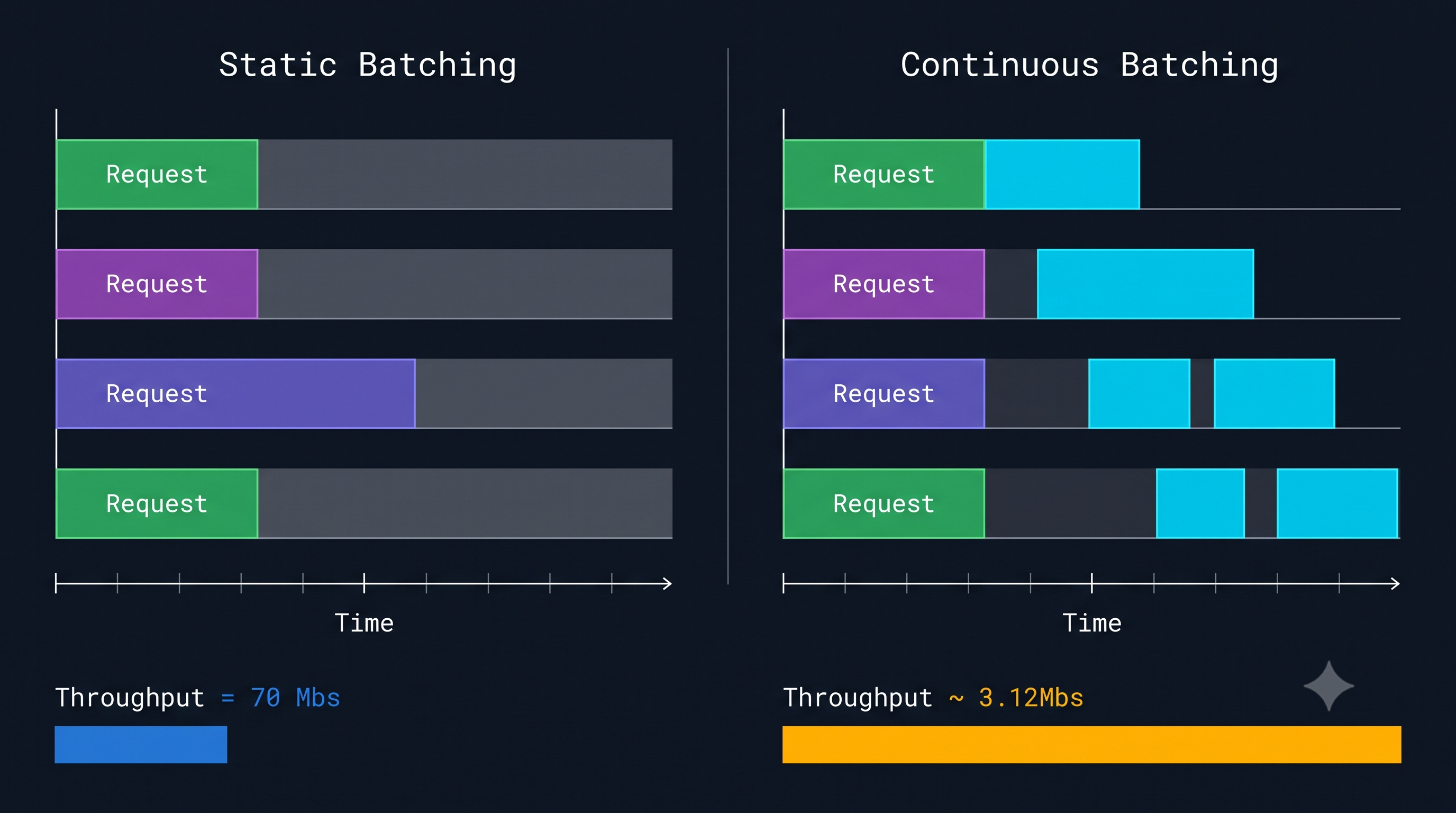
Throughput-bound systems (batch inference, synthetic data generation) maximize tokens generated per GPU-second. Here, PagedAttention’s fragmentation reduction and continuous batching (dynamically adding new sequences as others complete) are the primary levers. FP8 KV quantization provides another 2× headroom.

Cost-bound systems (research clusters, startup APIs) must minimize $/token. MLA adoption at architecture selection time provides the best long-term economics. Retrofit paths include aggressive KV quantization, CPU offload for distant context, and smaller KV head counts.

7. Minimal PyTorch Implementation

The following loop makes the cache mechanics concrete. This is not production code — it elides Flash Attention, GQA broadcasting, and batching — but it is mechanistically correct.

import torch
import torch.nn.functional as F

class CausalSelfAttentionWithKVCache(torch.nn.Module):
    def __init__(self, d_model: int, n_heads: int, max_seq_len: int):
        super().__init__()
        self.n_heads = n_heads
        self.head_dim = d_model // n_heads
        self.scale = self.head_dim ** -0.5

        self.W_Q = torch.nn.Linear(d_model, d_model, bias=False)
        self.W_K = torch.nn.Linear(d_model, d_model, bias=False)
        self.W_V = torch.nn.Linear(d_model, d_model, bias=False)
        self.W_O = torch.nn.Linear(d_model, d_model, bias=False)

        # KV cache: pre-allocated, grows in-place
        # Shape: [batch, n_heads, max_seq_len, head_dim]
        self.register_buffer('k_cache', torch.zeros(1, n_heads, max_seq_len, self.head_dim))
        self.register_buffer('v_cache', torch.zeros(1, n_heads, max_seq_len, self.head_dim))
        self.cache_len = 0  # current filled length

    def forward(self, x: torch.Tensor) -> torch.Tensor:
        """
        x: [batch, 1, d_model]  — single new token during autoregressive decode
        """
        B, T, D = x.shape
        assert T == 1, "This path is decode-only; use T=seqlen for prefill."

        # Project new token to Q, K, V
        q = self.W_Q(x).view(B, T, self.n_heads, self.head_dim).transpose(1, 2)
        k_new = self.W_K(x).view(B, T, self.n_heads, self.head_dim).transpose(1, 2)
        v_new = self.W_V(x).view(B, T, self.n_heads, self.head_dim).transpose(1, 2)

        # Append to cache — the core KV cache operation
        # k_new/v_new computed once per token; never recomputed
        self.k_cache[:, :, self.cache_len : self.cache_len + T, :] = k_new
        self.v_cache[:, :, self.cache_len : self.cache_len + T, :] = v_new
        self.cache_len += T

        # Attend over ALL past tokens using cached K, V
        k = self.k_cache[:, :, :self.cache_len, :]  # [B, H, t, head_dim]
        v = self.v_cache[:, :, :self.cache_len, :]  # [B, H, t, head_dim]

        # [B, H, 1, t] — Q is shape [B, H, 1, head_dim]
        attn_weights = torch.matmul(q, k.transpose(-2, -1)) * self.scale
        attn_weights = F.softmax(attn_weights, dim=-1)

        # [B, H, 1, head_dim]
        out = torch.matmul(attn_weights, v)
        out = out.transpose(1, 2).contiguous().view(B, T, D)
        return self.W_O(out)


# --- Autoregressive decode loop ---
def autoregressive_decode(model, prompt_tokens: torch.Tensor, max_new_tokens: int):
    """
    prompt_tokens: [1, seq_len]
    Prefill is handled separately (full sequence, no cache);
    this demonstrates the decode loop where KV cache eliminates O(t²) recomputation.
    """
    generated = []
    # Assume prefill already populated the cache up to prompt length
    x = prompt_tokens[:, -1:]  # last prompt token as first decode input

    for step in range(max_new_tokens):
        # Per-step cost: O(current_cache_len * head_dim), NOT O(t²)
        logits = model(x)               # [1, 1, vocab_size]
        next_token = logits[:, -1, :].argmax(dim=-1, keepdim=True)  # greedy
        generated.append(next_token)
        x = next_token  # feed generated token as next input

    return torch.cat(generated, dim=1)

The key line is the cache append: self.k_cache[:, :, self.cache_len:self.cache_len+T, :] = k_new. This is the entire insight materialized. One write. No recomputation. The subsequent matmul reads from cache — bandwidth-bound, not compute-bound, which is why KV cache dominates HBM utilization at long context.

8. Where This Is Heading

The trajectory is clear. Context windows are expanding faster than HBM capacity: GPT-4 at 128K, Gemini 1.5 at 1M, the architectural push toward perpetual context. The KV cache problem does not become easier at 1M tokens — it becomes existential.

MLA-style latent compression will likely become the dominant architectural primitive for the next generation of long-context models. PagedAttention (or its derivatives in SGLang and TensorRT-LLM) will remain the production-grade memory management layer. KV quantization will standardize at FP8, with INT4 becoming viable for V tensors as calibration techniques mature.

The deeper lesson is that memory architecture is not infrastructure — it is model design. Decisions made at the architecture selection stage (GQA vs MHA, MLA vs standard attention, head count, head dimension) determine production economics more than any post-hoc serving optimization. A senior ML engineer who understands the KV cache at this level can reason about model design choices, cluster sizing, and inference cost with a precision that no benchmark sheet provides.

The quadratic wall was never a compute problem. It was always a memory problem dressed in compute’s clothing.

References

Ainslie et al. (2023). GQA: Training Generalized Multi-Query Transformer Models from Multi-Head Checkpoints. arXiv:2305.13245
DeepSeek-AI (2024). DeepSeek-V2: A Strong, Economical, and Efficient Mixture-of-Experts Language Model. arXiv:2405.04434 (MLA introduced here)
Kwon et al. (2023). Efficient Memory Management for Large Language Model Serving with PagedAttention. arXiv:2309.06180 (vLLM)
Liu et al. (2024). KIVI: A Tuning-Free Asymmetric 2bit Quantization for KV Cache. arXiv:2402.02750
Dao et al. (2022). FlashAttention: Fast and Memory-Efficient Exact Attention with IO-Awareness. arXiv:2205.14135

BibTeX

@article{fp4-2606004,
  title   = {The KV Cache: A Definitive Engineering Analysis},
  author  = {fp4 editorial desk},
  year    = {2026},
  url     = {https://fp4.dev/system/kv-cache-engineering/},
  journal = {fp4}
}