01 — The Problem
GPU memory hierarchy explained: the reason your 70B model inference underperforms the theoretical peak by 10× is almost never the ALUs. It is the memory system. The H100 SXM5 delivers 3,958 TFLOPS of FP8 compute — a figure that appears in every press release. What appears less often is that the memory bandwidth to feed those units at full utilization is 3.35 TB/s from HBM3, which works out to roughly 0.85 bytes per FLOP. For a matrix-vector multiply (the dominant operation in decode), you need approximately 2 bytes per FLOP of memory traffic. The arithmetic ceiling is not the problem. The memory wall is.
This shapes every architectural decision downstream: which attention variant fits a given sequence length, why speculative decoding works, why continuous batching changes the economics, and why H200’s bandwidth bump matters more than its FLOPs bump for most production inference loads.
02 — Five Levels, Five Latencies
The H100’s memory subsystem is a five-level hierarchy, each with a different capacity/bandwidth/latency tradeoff:
| Level | Capacity | Bandwidth | Latency |
|---|---|---|---|
| Registers | 256 KB / SM | ~100 TB/s | ~1 cycle |
| L1 / Shared mem | 228 KB / SM (configurable) | ~30 TB/s | ~30 cycles |
| L2 cache | 50 MB | ~10 TB/s | ~200 cycles |
| HBM3 | 80 GB | 3.35 TB/s | ~600 cycles |
| NVLink / PCIe | — | 900 GB/s / 64 GB/s | ~5 µs |
The key insight: bandwidth drops by roughly 3× at each level boundary, while latency increases by 5–10×. A kernel that cannot hide memory latency with compute will stall.
03 — Roofline Analysis
The roofline model characterizes whether a kernel is compute-bound or memory-bound. For a given operation with arithmetic intensity (FLOPs per byte), peak performance (FLOPs/s) is:
where is memory bandwidth.
The ridge point for H100 with HBM3 is:
Any kernel with arithmetic intensity below 1,180 FLOPs/byte is memory-bound on H100. For comparison:
- GEMM (large batch): ~200–1,000 FLOPs/byte depending on tile size
- Attention (decode, single token): ~1–4 FLOPs/byte — deeply memory-bound
- LayerNorm / elementwise ops: ~2–10 FLOPs/byte — memory-bound
- Large dense GEMM (prefill): ~500–2,000 FLOPs/byte — can be compute-bound
This is why decode is fundamentally different from prefill. During decode you process one token against all KV cache entries — the operation is memory-bandwidth-bound. During prefill you process the entire prompt at once — sufficiently large batch sizes make it compute-bound.
04 — Shared Memory and Tiling
Kernels improve arithmetic intensity by tiling: loading a block of data into shared memory (L1, 228 KB on H100), reusing it across many operations before going back to HBM. A tiled GEMM with tile size achieves:
For 32-bit floats. At , FLOPs/byte — still memory-bound but ~64× better than an untiled kernel. At BF16 (), it reaches ~128 FLOPs/byte. Still below the ridge point, but approaching it for large-batch prefill.
This is the logic behind FlashAttention. Rather than materializing the full attention matrix in HBM — which requires memory bandwidth — it tiles the computation entirely in shared memory, trading recomputation during the backward pass for dramatically reduced HBM traffic. The FlashAttention-2 paper shows this achieves 2–4× speedup for sequence lengths ≥ 1024.
# Simplified tiled attention (pseudocode, not production)
# Full implementation: https://github.com/Dao-AILab/flash-attention
import torch

def flash_attention_naive_tiled(Q, K, V, block_size=64):
    B, H, N, d = Q.shape
    O = torch.zeros_like(Q)
    L = torch.zeros(B, H, N, 1, device=Q.device)

    for i in range(0, N, block_size):
        q_block = Q[:, :, i:i+block_size]          # load from HBM once
        acc = torch.zeros_like(q_block)
        l_acc = torch.zeros(B, H, block_size, 1, device=Q.device)

        for j in range(0, N, block_size):
            k_block = K[:, :, j:j+block_size]       # tile K in SRAM
            v_block = V[:, :, j:j+block_size]       # tile V in SRAM
            s = torch.einsum('bhid,bhjd->bhij', q_block, k_block)
            s = s / (d ** 0.5)
            p = torch.exp(s - s.amax(dim=-1, keepdim=True))
            acc += torch.einsum('bhij,bhjd->bhid', p, v_block)
            l_acc += p.sum(dim=-1, keepdim=True)

        O[:, :, i:i+block_size] = acc / l_acc

    return O
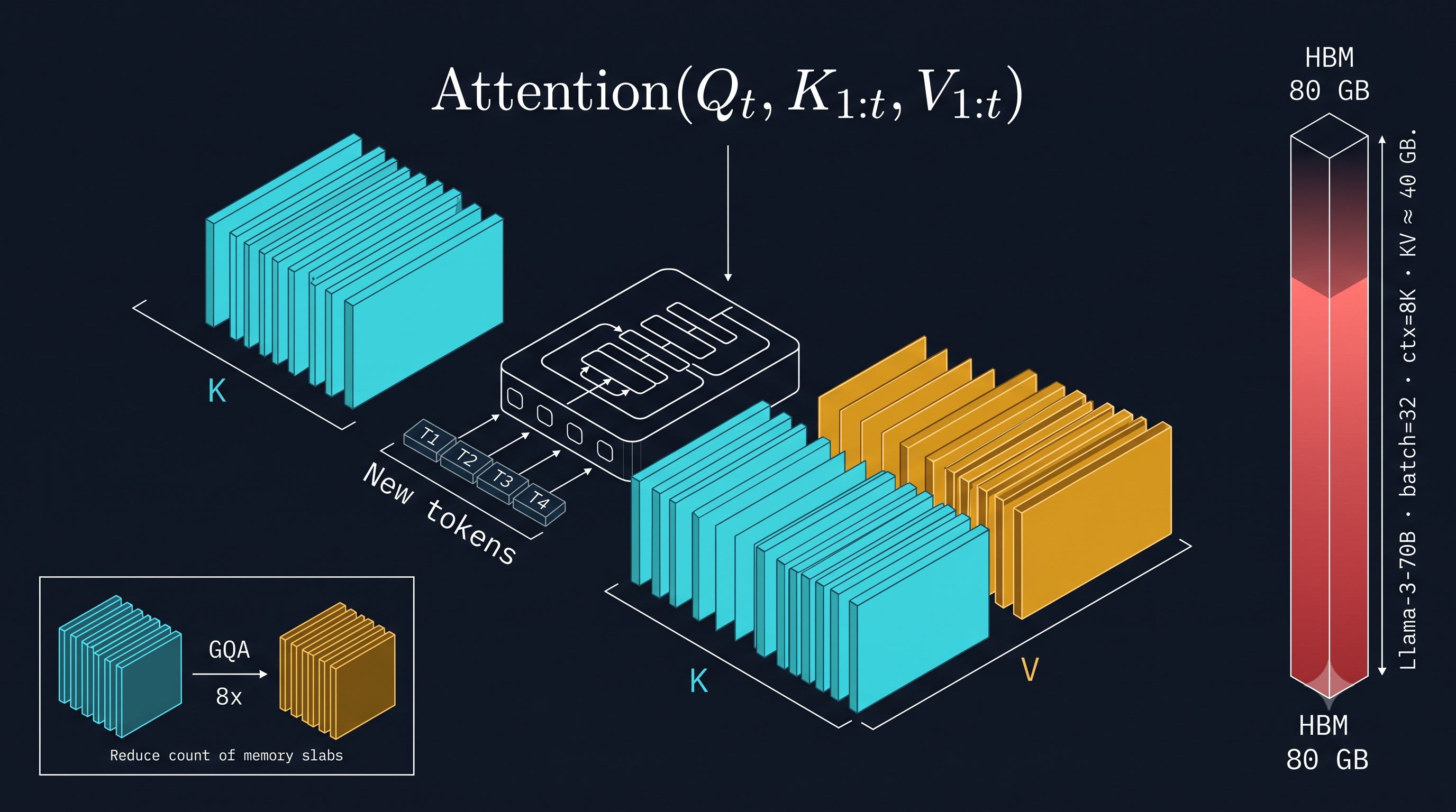
05 — HBM Bandwidth and Inference Economics
For single-token decode, the operation per layer is a matrix-vector multiply: weight matrix against a single activation vector. For Llama-3-70B (, ), one feed-forward layer requires:
at BF16. Across 80 layers (8B model) or 80 layers (70B model), the total weight traffic per token is in the range of 140 GB for a 70B model. At H100 HBM bandwidth of 3.35 TB/s, the minimum time per token is:
That is ~24 tokens/second maximum for single-batch inference, purely from memory bandwidth. This is why batching is critical: with batch size , the same weights serve tokens simultaneously, and throughput scales linearly until you hit a different bottleneck (KV cache memory, or eventually compute).
For a deeper treatment of the inference economics and hardware tradeoffs, see H100 vs H200 vs B200 TCO — the B200’s 8 TB/s bandwidth changes this picture significantly. For the interconnect implications in multi-GPU inference, see distributed interconnects.
References
- [1] Dao et al.. FlashAttention: Fast and Memory-Efficient Exact Attention with IO-Awareness . NeurIPS, 2022. arXiv:2205.14135.
- [2] Dao. FlashAttention-2: Faster Attention with Better Parallelism and Work Partitioning . ICLR, 2024. arXiv:2307.08691.
- [3] Williams et al.. Roofline: An Insightful Visual Performance Model for Multicore Architectures . Communications of the ACM, 2009. arXiv:2212.09561.
BibTeX
@article{fp4-2606001,
  title   = {GPU Memory Hierarchy and Kernel Performance},
  author  = {fp4 editorial desk},
  year    = {2026},
  url     = {https://fp4.dev/silicon/gpu-memory-hierarchy/},
  journal = {fp4}
}