01 — The Problem
Distributed interconnects explained: the practical question when training a model that doesn’t fit on a single GPU is not “how do I shard it?” but “can the interconnect keep up with the compute?” A DGX H100 node with 8 GPUs delivers 134 petaFLOPS of BF16 throughput. NVLink 4.0 connecting those GPUs delivers 900 GB/s bidirectional bandwidth. The ratio determines your scalable efficiency ceiling before you even write the first line of training code.
This article maps the full interconnect stack — from NVLink bisection bandwidth inside a node to InfiniBand and RoCE across nodes — and derives the collective communication overhead that limits large-scale training runs.
02 — Intra-node: NVLink and NVSwitch
NVLink 4.0 (H100) provides 900 GB/s total bidirectional bandwidth per GPU, organized as 18 NVLink 4.0 lanes at 50 GB/s each. In an 8-GPU DGX H100, all GPUs connect through the NVSwitch fabric — a full non-blocking all-to-all topology where any GPU can reach any other GPU at full NVLink speed.
The effective all-reduce bandwidth for an -GPU all-reduce via ring algorithm is:
For and GB/s (unidirectional):
In practice, NCCL achieves 650–700 GB/s effective all-reduce throughput on large tensors within a single DGX H100 node, primarily due to NVSwitch fabric overhead and NCCL tree/ring switching heuristics.
For comparison, a PCIe 5.0 × 16 link (the alternative for systems without NVSwitch) delivers 64 GB/s bidirectional — a 14× bandwidth reduction that effectively caps tensor-parallel scale to 2 GPUs before communication dominates.
03 — Inter-node: InfiniBand vs RoCE
Across nodes, two technologies dominate:
InfiniBand NDR (2024): 400 Gbps per port, 800 Gbps with dual-port NICs. Full lossless fabric with hardware-level credit-based flow control. RDMA native. Latency: 600 ns port-to-port. The standard for hyperscaler training clusters (Meta RSC, Google TPU pods use equivalent, Microsoft Azure NDv5).
RoCE v2: RDMA over Converged Ethernet. 400 Gbps per port (ConnectX-7 with 400GbE). Requires PFC (Priority Flow Control) + ECN (Explicit Congestion Notification) for lossless operation. Latency: 1–3 µs port-to-port. ~40% cheaper than IB at the NIC level; switch costs are lower because Ethernet switches are commoditized. Used by AWS EFA (Elastic Fabric Adapter), which is essentially RoCE with proprietary congestion control.
The bandwidth hierarchy per node:
| Level | Technology | BW (bidirectional) | Latency |
|---|---|---|---|
| GPU↔GPU (intra) | NVLink 4.0 | 900 GB/s | ~1 µs |
| Node↔Node (NDR IB) | InfiniBand NDR | 100 GB/s (800 Gbps) | ~2 µs |
| Node↔Node (RoCE) | RoCE v2 / EFA | 100 GB/s (800 Gbps) | ~4 µs |
| Node↔Node (PCIe+IB) | No NVSwitch | 50 GB/s | ~5 µs |
The inter-node gap is a 9× bandwidth reduction from intra-node NVLink. This is the fundamental constraint on pipeline parallelism bubble overhead and gradient synchronization frequency.
04 — Collective Operation Costs
The four NCCL collectives that dominate distributed training:
# Time complexity for key collectives (ring algorithm, N nodes, M bytes)
# These are theoretical; NCCL has tree/ring hybrids above certain thresholds

def allreduce_time(N, M, bw_gbps):
    """Ring all-reduce: 2*(N-1)/N * M / BW"""
    return 2 * (N - 1) / N * M / (bw_gbps * 1e9)

def allgather_time(N, M, bw_gbps):
    """Ring all-gather: (N-1)/N * M / BW"""
    return (N - 1) / N * M / (bw_gbps * 1e9)

def reducescatter_time(N, M, bw_gbps):
    """Ring reduce-scatter: (N-1)/N * M / BW"""
    return (N - 1) / N * M / (bw_gbps * 1e9)

# Example: all-reduce of 1 GB gradient across 8 nodes (IB NDR, 100 GB/s)
t = allreduce_time(N=8, M=1e9, bw_gbps=100)
# t ≈ 17.5 ms per all-reduce across 8 nodes
For a 70B parameter model with BF16 gradients (140 GB total), a full gradient all-reduce across 8 nodes at 100 GB/s takes:
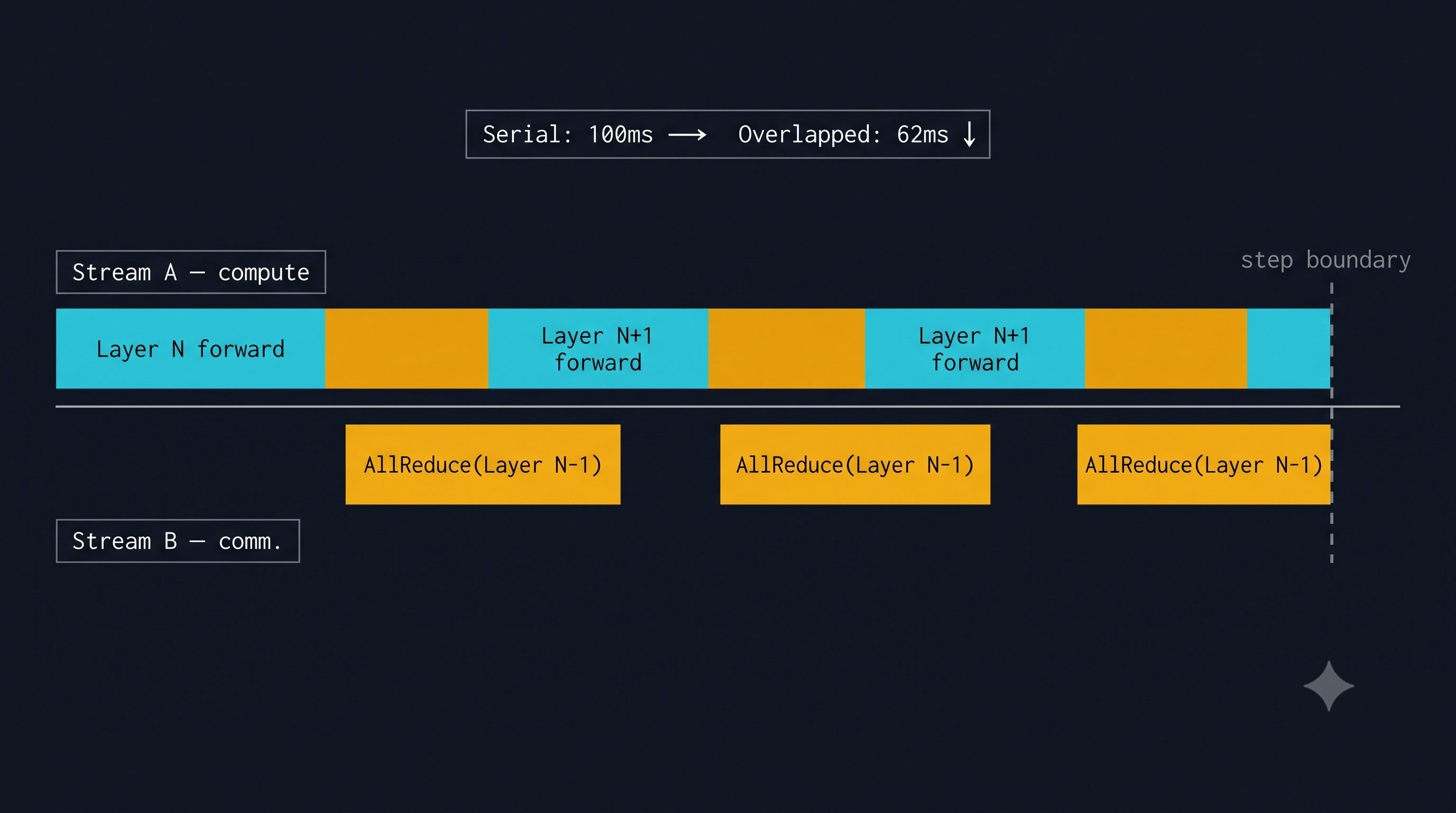
A forward+backward pass on the same model with H100 takes approximately 1.5–3s depending on sequence length and batch size. So gradient synchronization is the same order of magnitude as compute — which is why gradient compression, pipeline parallelism, and ZeRO-3 optimizer state sharding exist.
05 — Parallelism Strategy Selection
The interconnect bandwidth directly determines which parallelism strategy is viable:
Tensor Parallelism (TP): Requires all-reduce at every transformer layer. Latency-sensitive: high-bandwidth, low-latency communication (NVLink) essential. Practical TP degree: ≤ 8 (within a single node). Cross-node TP is theoretically possible but communication overhead typically makes it inefficient unless using InfiniBand NDR with SHARP in-network compute.
Pipeline Parallelism (PP): Point-to-point activation passing between pipeline stages. Bandwidth requirement is much lower (one activation tensor per micro-batch, not all gradients). Can span nodes. The cost is pipeline bubbles: for pipeline depth and micro-batches , bubble fraction is .
Data Parallelism (DP) / FSDP / ZeRO: Gradient all-reduce (DP) or optimizer state sharding (FSDP/ZeRO). Bandwidth requirement scales with model size. ZeRO-3 reduces per-GPU memory by factor at the cost of 3× the all-reduce bandwidth of vanilla DP.
The standard recipe for 70B–405B scale training: TP=8 within node (NVLink), PP=4–8 across nodes (IB/RoCE), DP over the remaining dimension. This maximizes NVLink utilization for the most latency-sensitive collective (TP all-reduce) while tolerating inter-node latency in pipeline micro-batch passing.
For the hardware-level details of why HBM bandwidth determines decode throughput, see GPU memory hierarchy. For infrastructure-level TCO implications of choosing IB vs RoCE in an H100 cluster, see H100 vs H200 vs B200 TCO.
References
- [1] Rajbhandari et al.. ZeRO-Infinity: Breaking the GPU Memory Wall for Extreme Scale Deep Learning . SC, 2021. arXiv:2104.12212.
- [2] Narayanan et al.. Efficient Large-Scale Language Model Training on GPU Clusters Using Megatron-LM . SC, 2021. arXiv:2205.05198.
- [3] Ying et al.. Image Classification at Supercomputer Scale . 2018. arXiv:1811.05233.
BibTeX
@article{fp4-2606002,
  title   = {Intra-node vs Inter-node Interconnects in Distributed Training},
  author  = {fp4 editorial desk},
  year    = {2026},
  url     = {https://fp4.dev/system/distributed-interconnects/},
  journal = {fp4}
}