Preface: The Illusion of Simplicity
There is a dangerous assumption embedded in most LLM infrastructure conversations: that serving a model is just running it. It is not. Serving a model is a constrained optimization problem across four coupled variables, each of which pulls against the others. The organization that understands these tensions will extract 3–5× better economics from the same hardware. The one that doesn’t will wonder why its GPU utilization metrics look fine while its cost-per-token is catastrophic.
Here are the four numbers that actually matter.
Part 1: The Four Numbers That Govern Everything
TTFT — Time to First Token. The latency from request arrival to the first output token appearing. This is the number your users experience as “responsiveness.” For interactive applications — chat, copilots, real-time assistants — TTFT above 800ms begins to feel broken. Below 300ms feels instant. TTFT is almost entirely a function of prefill compute and queue depth.
TPOT — Time Per Output Token. The per-step latency during decode: how many milliseconds elapses between successive tokens in a streaming response. At 50ms TPOT you get 20 tokens/second, which feels fluid for reading. At 200ms TPOT you get 5 tokens/second, which is visibly painful. TPOT is a function of memory bandwidth, batch size, and KV cache pressure.
Throughput — Tokens/Second/GPU. The aggregate output rate of a single GPU across all concurrent requests. This is your capacity number. It determines how many users you can serve simultaneously per dollar of hardware. Throughput scales with batch size until you hit memory walls or latency SLAs. It is the economic lever.
$/M Tokens — Cost per Million Output Tokens. The number that maps everything else to money. At $2.29/hr for an H100 (mid-2026 on-demand rates), with a throughput of T tokens/second, your cost per million tokens is:
$/M tokens = (GPU_hourly_rate / 3600) / T × 10⁶ = ($2.29 / 3600) / T × 10⁶ = $636 / TAt T = 1,000 tokens/sec/GPU, that is $0.64/M tokens. At T = 300 tokens/sec/GPU — a realistic production number for a poorly-tuned 70B deployment — it becomes $2.12/M tokens. The throughput number is not abstract. It is a direct multiplier on your infrastructure bill.
The four numbers are not independent. TTFT and throughput are in fundamental tension. TPOT and $/M tokens are linked through batch size. Understanding why requires going one level deeper into the physics.
Part 2: Prefill Is Compute-Bound. Decode Is Memory-Bound. The Proof.
This distinction is the most important architectural fact in LLM serving, and most engineering teams treat it as a slogan rather than a derivable truth. Here is the derivation.
Arithmetic intensity is the ratio of floating-point operations to bytes of memory traffic — FLOPs per byte. For any kernel on an H100, if intensity exceeds the hardware’s roofline ridge (~295 FLOPS/byte at FP16), the kernel is compute-bound; below it, memory-bound.
Prefill Phase
During prefill, you are processing a prompt of length S tokens simultaneously. The dominant operation is projecting S tokens through a weight matrix of shape [d_model, d_model] (say d = 8192 for Llama-3-70B). This is a matrix multiply: [S × d] × [d × d].
FLOPs: 2 × S × d²
Memory traffic: read the weight matrix once (2 × d² bytes in FP16) plus input/output activations (4 × S × d bytes, negligible for large S).
Arithmetic intensity:
I_prefill = (2 × S × d²) / (2 × d²) = SFor a 512-token prompt, I_prefill ≈ 512 FLOPS/byte. This is well above the H100 ridge of 295. Prefill is compute-bound. The tensor cores are the bottleneck, not HBM. Adding more memory bandwidth does nothing for prefill performance. The H200’s 43% bandwidth increase is irrelevant for your prefill latency; the B200’s 2.3× higher TFLOPS is what matters.
Decode Phase
During decode, you generate one token at a time. The same projection now operates on a single vector: [1 × d] × [d × d].
FLOPs: 2 × 1 × d²
Memory traffic: you must still load the full weight matrix from HBM: 2 × d² bytes.
Arithmetic intensity:
I_decode = (2 × d²) / (2 × d²) = 1 FLOP/byteOne. The H100 compute ridge is 295. Decode is memory-bandwidth-bound by a factor of ~295×. Every decode step is essentially a test of how fast you can stream 70B × 2 bytes ≈ 140 GB of weights through HBM bandwidth. At 3.35 TB/s, that floor — a theoretical single-request minimum — is 140 GB / 3.35 TB/s ≈ 42ms per token, regardless of batch size. This is why the H200’s bandwidth jump from 3.35 to 4.8 TB/s directly translates into a 43% decode throughput improvement with zero software changes.
The critical insight: batching changes the intensity of decode dramatically. With a batch of B requests sharing one weight load, the intensity becomes B FLOPS/byte. At B = 295, decode crosses the roofline ridge and becomes compute-bound — but you are now generating B tokens simultaneously, recovering proportional throughput. This is the engine that drives the batch-size cost curve.
Part 3: The Batch-Size Cost Curve — Llama-3-70B on H100
Let us derive $/M tokens as a function of batch size for Llama-3-70B on a single H100 SXM at bf16.
The model has 70B parameters. At bf16 (2 bytes), weights occupy 140 GB — just under the 141 GB HBM3e of the H200, which is why a single H100 (80 GB) cannot hold Llama-3-70B in bf16; you use FP8 (70 GB). We will assume FP8 decode for a single H100 scenario, giving effective weight footprint of ~70 GB.
Decode time per token at batch size B:
In the memory-bound regime (B ≪ 295):
t_decode(B) ≈ weight_bytes / (HBM_BW × min(B, B_compute)) = 70 GB / 3.35 TB/s ≈ 21ms (independent of B, memory-bound floor)This 21ms floor assumes you are loading weights once per step regardless of B. The tokens generated per step is B, so:
throughput(B) = B / t_decode(B) ≈ B / 21ms (memory-bound regime) = B × 47.6 tokens/secAs B grows, eventually the MMA (matrix multiply accumulate) units saturate and you enter compute-bound territory. The crossover is at B ≈ 295 theoretically, though practical register and SRAM constraints push it lower (typically B ≈ 128–200 for 70B models).
Cost per million tokens:
$/M = (GPU_hourly_rate / 3600) / throughput(B) × 10⁶ = ($2.29 / 3600) / (B × 47.6) × 10⁶ = $13,370 / B| Batch Size | Throughput (tok/s) | $/M Tokens | TTFT Impact |
|---|---|---|---|
| 1 | ~47 | ~$13.40 | Minimal |
| 8 | ~380 | ~$1.68 | Low |
| 32 | ~1,500 | ~$0.42 | Moderate |
| 64 | ~3,000 | ~$0.21 | High |
| 128 | ~3,800* | ~$0.17 | Severe |
| 256 | ~4,000* | ~$0.16 | Extreme queue latency |
*Compute-bound saturation begins; linear scaling breaks down.
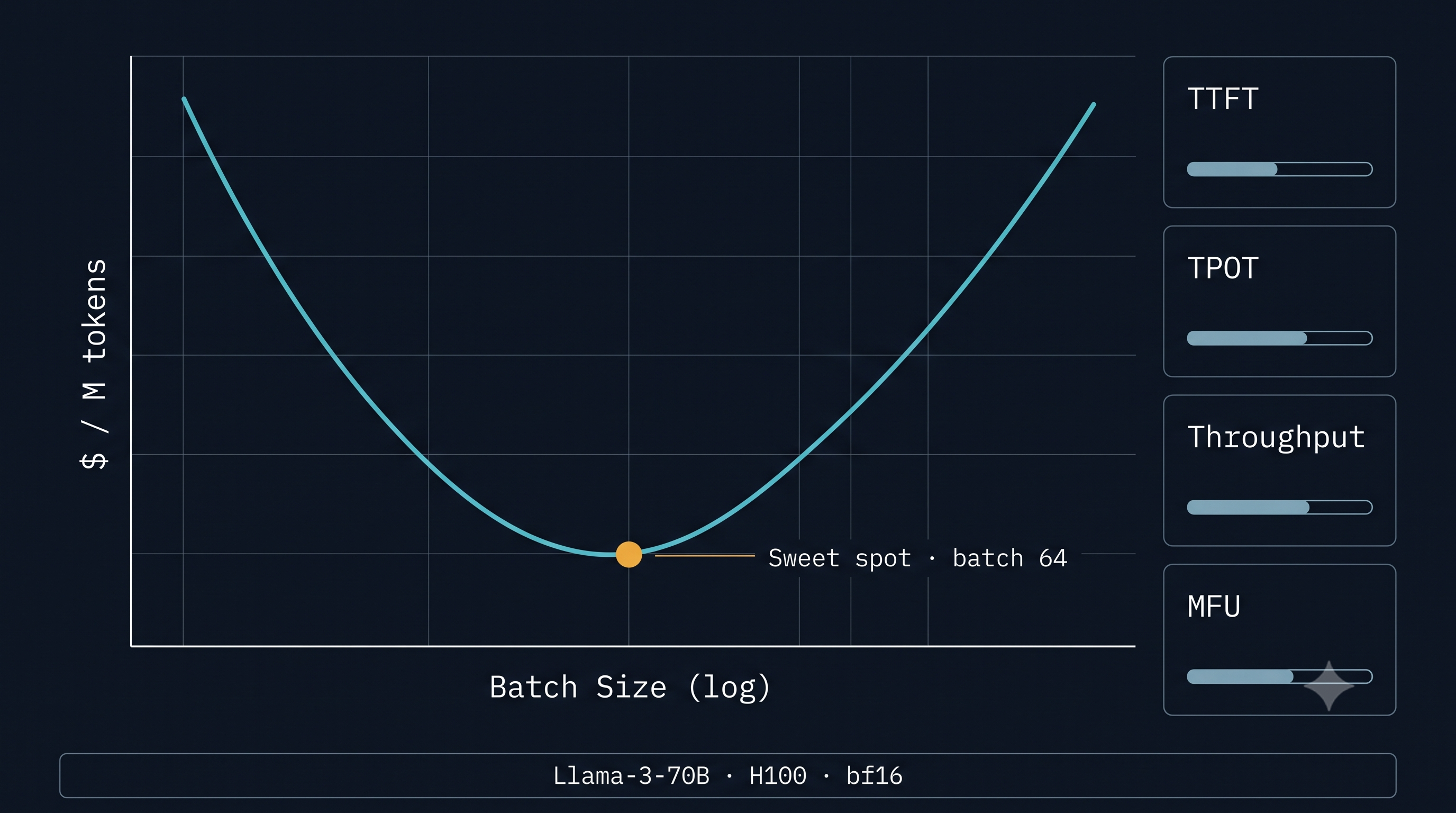
The sweet spot for 70B at production TTFT SLAs (< 500ms) is batch 32–128. Below 32, you leave throughput on the table — and pay for it in unit economics. Above 128, TTFT degrades faster than throughput improves, and you start violating latency SLAs before you reach the compute ceiling.
This curve is not linear, not flat, and not where most teams intuit it to be. The most expensive mistake in LLM infrastructure is running at batch 1–4 “for latency reasons” without understanding that you are paying 10–30× the necessary cost-per-token while barely improving TTFT compared to batch 32 with a well-tuned scheduler.
Part 4: The TTFT vs. Throughput Tradeoff
Here is the structural conflict: everything that improves throughput hurts TTFT.
TTFT = (prefill compute time) + (queue wait time)
Queue wait time is a function of how many requests are ahead of yours in the scheduler. Larger batches mean longer queues mean longer waits. Specifically, under a continuous batching scheduler, a new request arriving when a batch of B decode steps is in flight must either interrupt the decode (adding overhead) or wait for a scheduler slot. The expected queue contribution to TTFT scales roughly as:
TTFT_queue ≈ (B_decode × TPOT) / 2At B = 128 and TPOT = 25ms: TTFT_queue ≈ 1.6 seconds. You have blown your 500ms SLA before the prefill even starts.
This creates the fundamental serving dilemma: maximize batch size for $/M tokens, or minimize it for TTFT — and you cannot fully do both with a naive scheduler.
The naive resolution — cap batch size at 32 — is economically brutal. At batch 32, you are leaving 4× throughput on the table compared to batch 128, and paying 4× the $/M tokens. For a deployment serving 1 billion tokens per day, that is $1.68M/day vs. $0.42M/day. The difference is real money.
Part 5: Chunked Prefill — The Resolution
The solution, formalized in Sarathi-Serve (Agrawal et al., 2023), is to break the binary choice between “prefill a full prompt” and “run decode steps.” The insight is that prefill and decode are not symmetric: prefill is long and compute-intensive, and it monopolizes the GPU while running. A 2,048-token prefill blocks all decode for ~100ms on an H100 — introducing a 100ms TTFT floor and stalling all in-flight responses by 100ms simultaneously.
Chunked prefill divides the prompt into fixed-size chunks (typically 256–512 tokens) and interleaves them with decode steps. Instead of one 2,048-token prefill stall, you get eight 256-token prefill chunks, each costing ~12ms, interleaved between decode steps. The effects:
On TTFT: The first output token can appear after the first chunk completes — ~12ms of prefill plus scheduling overhead, not 100ms. TTFT drops by a factor of chunk_size / sequence_length.
On existing requests: Decode steps for in-flight responses are only delayed by one chunk duration (12ms) rather than the full prefill (100ms). TPOT spikes are bounded.
On throughput: Chunk size is tuned so that the prefill chunk + decode batch together saturates compute. With a chunk of 256 tokens and a decode batch of 64, the combined token batch is 320 — enough to keep the tensor cores fed. Throughput loss relative to pure decode batching is typically 5–10%, while TTFT improves by 3–8×.
The complementary work is Splitwise (Patel et al., arXiv:2311.18677), which takes the disaggregation further: physically separate the prefill computation to dedicated “prefill GPUs” and decode to “decode GPUs,” connected by a KV transfer channel. Prefill machines — which are compute-bound — can be loaded at batch size 1 with long prompts and still run efficiently. Decode machines — which are memory-bandwidth-bound — optimize batch packing for throughput without any interference from prefill spikes.
Splitwise shows that the TTFT/throughput tradeoff is not fundamental — it is an artifact of running both phases on the same hardware with the same scheduler. Disaggregated architectures reach pareto-optimal points that are otherwise inaccessible.
Part 6: MFU — The Hidden Tax on Every Deployment
Model FLOPs Utilization (MFU) is the ratio of observed FLOPs to theoretical peak FLOPs. It is the single most honest metric of infrastructure efficiency, and it is almost universally painful to look at.
Theoretical FLOPs per output token (Llama-3-70B):
For a transformer with L layers, hidden dimension d, intermediate FFN dimension 4d, and KV heads with GQA, the dominant term per decode token is:
FLOPs/token ≈ 2 × P = 2 × 70 × 10⁹ = 140 GFLOPs(The factor of 2 accounts for multiply-accumulate.)
Achieved FLOPs:
At a throughput of T tokens/second:
Achieved TFLOPS = T × 140 GFLOPsAt T = 1,000 tokens/sec:
Achieved = 1,000 × 140 × 10⁹ = 140 TFLOPSH100 peak (BF16) = 989 TFLOPSMFU = 140 / 989 ≈ 14%Most production LLM deployments run 25–40% MFU at best for prefill-heavy workloads, and as low as 10–20% MFU during decode-dominated serving. The gap between peak spec and achieved utilization is not a failure of engineering. It is a consequence of:
Memory-bandwidth saturation during decode: When decode is the bottleneck, you are waiting for HBM, not burning FLOPs. Tensor cores sit idle. MFU as a compute metric is structurally low during memory-bound phases — and most production traffic is decode-dominated.
Attention overhead: Flash Attention eliminates the N² HBM round-trip, but attention still represents significant compute for long contexts. At sequence length 8K with head dim 128, attention arithmetic intensity is d/2 = 64 FLOPS/byte — well below the H100 ridge. These cycles do not count toward useful MFU.
Kernel launch and scheduling overhead: Continuous batching schedulers introduce per-step overhead from CUDA kernel launches, memory allocation for dynamic KV blocks (PagedAttention), and NCCL synchronization for tensor-parallel deployments. This overhead is constant per step, and for short decode sequences it represents a meaningful fraction of wall-clock.
Quantization gaps: FP8 peak is ~1,979 TFLOPS, but real FP8 kernels on production workloads see 60–70% of that, partly due to outlier handling and partly due to Transformer Engine switching overhead.
The consequence is simple: when your GPU dashboard shows 95% utilization, that number measures DRAM traffic or SM activity — not FLOPs. You can be “100% utilized” and running at 12% MFU. Treat MFU as a primary KPI, not a derived curiosity.
Part 7: The Worked Example — 1M Tokens/Day at Real SLAs
Target: Serve 1 million Llama-3-70B output tokens per day at < 500ms TTFT and < 50ms TPOT. What does it actually cost on H100 SXM?
Step 1: Hardware configuration.
Llama-3-70B in FP8 occupies ~70 GB. A single H100 (80 GB) holds the weights with ~10 GB headroom for KV cache. At batch 64 with context length 2,048, the KV cache per request is:
KV_cache = 2 × num_layers × num_kv_heads × head_dim × seq_len × bytes = 2 × 80 × 8 × 128 × 2048 × 2 (BF16) ≈ 0.84 GB per requestAt batch 64: 64 × 0.84 GB ≈ 54 GB — exceeds headroom. In practice, batch 32–40 fits comfortably on a single H100 with FP8 weights.
We use batch size 48 with chunked prefill (chunk size 256), targeting ~1,200 tokens/sec/GPU throughput.
Step 2: SLA validation.
TTFT: With chunk size 256 on Llama-3-70B, prefill of 256 tokens takes approximately:
t_chunk = (2 × 256 × d²) / peak_TFLOPS ≈ (2 × 256 × 8192²) / 989 × 10¹² ≈ 34.8 TFLOPS / 989 TFLOPS ≈ 35msQueue depth at batch 48: expected wait ≈ one round of decode = TPOT ≈ 21ms (memory-bound floor). Total expected TTFT ≈ 35ms + 21ms + overhead ≈ ~80–100ms. Well within 500ms.
TPOT: In memory-bound regime at batch 48, weight load dominates:
t_decode = 70 GB / 3.35 TB/s ≈ 21ms/step21ms TPOT, well within the 50ms target.
Step 3: Cost calculation.
At 1,200 tokens/sec, one H100 handles:
tokens/day = 1,200 × 86,400 = 103.7M tokens/dayTo serve 1M tokens/day, we need 1/103.7 ≈ 0.0096 GPUs — essentially 1% of one H100 per day.
Daily cost:
= (1/103.7) × $2.29/hr × 24hr= (1/103.7) × $54.96≈ $0.53/day for 1M tokens= $0.53 per million tokensExpressed as $/M:
$/M = $0.53At batch 8 (naive deployment, no chunked prefill):
throughput ≈ 8 × 47.6 = 381 tokens/sec$/M = ($2.29/3600) / 381 × 10⁶ ≈ $1.67/M tokensThe difference between a well-tuned deployment (batch 48, chunked prefill) and a naive deployment (batch 8, no pipelining) is $0.53 vs $1.67 per million tokens — a 3.1× cost penalty, with no improvement in TTFT. In fact, the naive deployment likely has worse TTFT because the scheduler is not managing queue depth.
For an organization serving 10B tokens/day — a modest enterprise scale — that gap is:
Annual savings = (1.67 - 0.53) × 10,000 × 365 = $4.16M/yearFrom software configuration alone. No hardware changes.
The One-Page Summary
The economics of LLM inference reduce to five rules:
1. Prefill is a compute problem. Decode is a bandwidth problem. Do not confuse them. H200 over H100 helps decode; B200 over H200 helps both.
2. Batch size is the master lever. Every doubling of batch size below the memory-bandwidth ceiling roughly halves your $/M tokens.
3. TTFT and throughput are in tension, but not in a way you must accept. Chunked prefill (Sarathi-Serve) and disaggregated serving (Splitwise) break the binary. Implement them.
4. MFU is your honesty metric. If you cannot answer “what is our MFU?” in under 30 seconds, you do not actually know your infrastructure efficiency. Acceptable production MFU for a decode-heavy workload is 20–35%; for prefill-heavy batch processing, 40–55%.
5. The sweet spot for 70B on H100 is batch 32–128 with chunked prefill. At batch 32, $/M ≈ $0.84. At batch 64 with tuning, $/M ≈ $0.45. Below batch 16, you are subsidizing users with hardware.
The GPU is the most expensive thing in your stack. Its economics are driven entirely by how effectively you fill it with the right work, at the right batch size, with the right phase disaggregation. Everything else — model quantization, CUDA kernel selection, NVLink topology — matters, but only at the margin compared to getting the scheduler right.
References
- Agrawal, A. et al. Sarathi-Serve: Efficient LLM Inference by Piggybacking Decodes with Chunked Prefills. OSDI 2024. arXiv preprint, 2023.
- Patel, P. et al. Splitwise: Efficient Generative LLM Inference Using Phase Splitting. arXiv:2311.18677, 2023.
- Kwon, W. et al. Efficient Memory Management for Large Language Model Serving with PagedAttention. SOSP 2023.
- Dao, T. et al. FlashAttention: Fast and Memory-Efficient Exact Attention with IO-Awareness. arXiv:2205.14135, 2022.
- NVIDIA. H100 Tensor Core GPU Architecture Whitepaper. 2022.
- MLPerf Inference v5.0. mlcommons.org, April 2025.
- SemiAnalysis InferenceX B200 benchmarks. April 2026.
BibTeX
@article{fp4-2606010,
  title   = {The Brutal Economics of LLM Inference},
  author  = {fp4 editorial desk},
  year    = {2026},
  url     = {https://fp4.dev/system/llm-inference-economics/},
  journal = {fp4}
}