
You are building a platform where users onboard their own MCP and custom tools, define their own agents on shared LLM infrastructure, and where you — not the user — pay the API invoice. This is the engineering brief for making that economically survivable and behaviorally correct. It is dense on purpose. Every section is meant to be implemented, not admired.
01 — The Multi-Agentic Platform context crisis
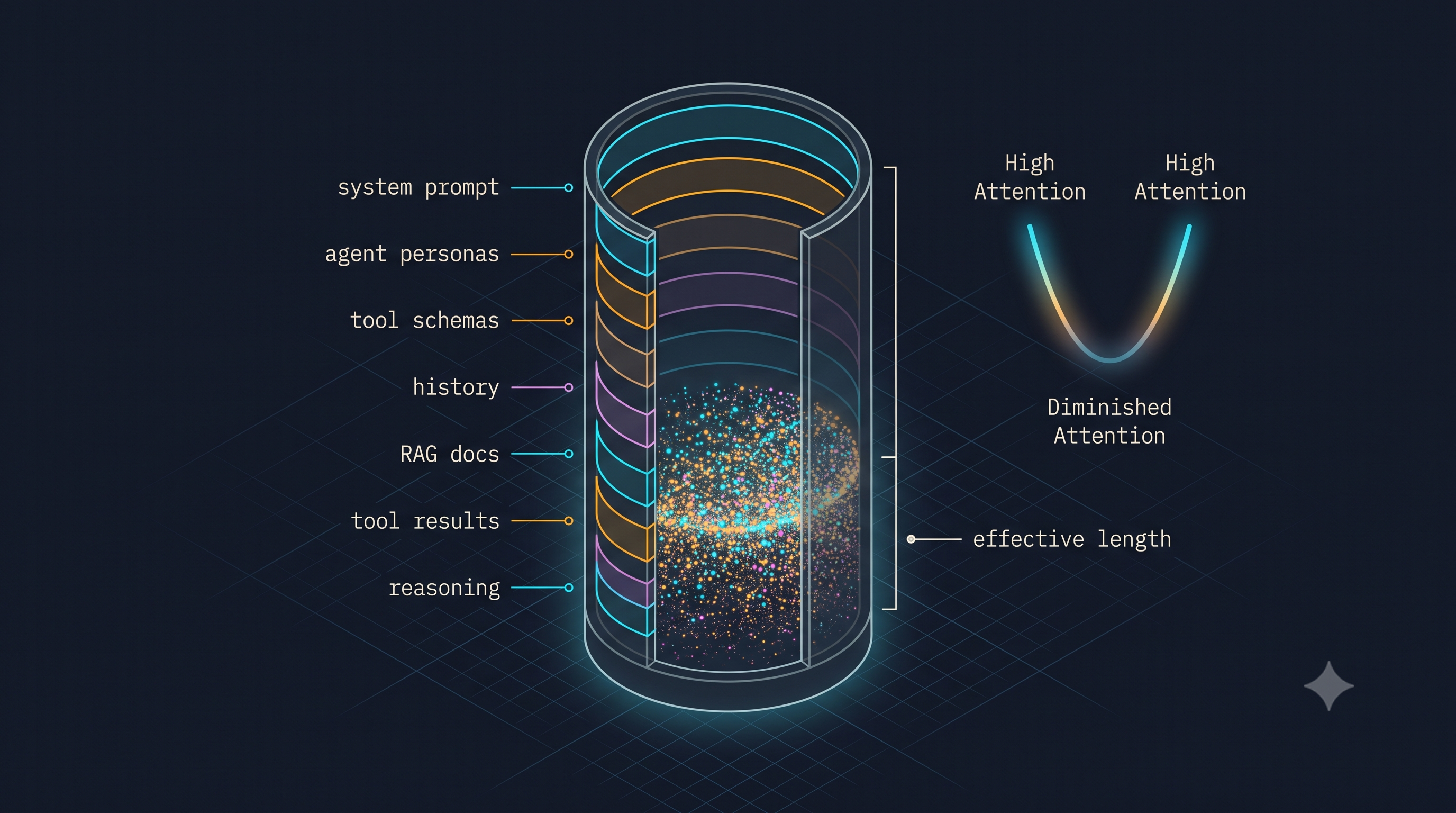
A single-user chatbot has exactly one thing eating its context window: the conversation. A Multi-Agentic Platform has seven, and they compound multiplicatively because the platform, not the user, chose to make tools onboardable, agents definable, and infrastructure shared. Every one of those product decisions is a standing charge against a finite window that you refill on every turn.
| Layer | Per-turn cost | Growth driver |
|---|---|---|
| Base platform system prompt | 1–3K | Fixed, stable, cacheable |
| Custom agent persona / instructions (per active agent) | 1–3K each | Scales with active agents |
| Onboarded MCP / custom tool descriptions | 200–1,500 per tool | Scales with onboarded tools |
| Conversation history | unbounded | Every turn |
| Retrieved documents (RAG) | 2–20K per turn | Often re-injected verbatim |
| Tool call results / observations | 500–5,000 per tool use | Raw JSON is the silent killer |
| Reasoning / extended-thinking traces | 5–50K per hard problem | Reasoning models |
Worked example. A user has 20 MCP tools onboarded, 3 active personas, and is on turn 5. Tool descriptions alone run ~24K (20 × ~1.2K). Three personas add ~6K, the base prompt ~2K, five turns of history plus a couple of RAG pulls and tool observations reach ~55K. That is ~87K tokens consumed before the model emits a single output token — 44% of a 200K window spent on scaffolding. Users report this as “the AI got confused.” It is not confusion; it is context pressure, and it is measurable.
Formally, context consumed at turn t is:
The entire discipline of this guide is that every right-hand term is independently bounded and independently optimizable. is cached. is scoped to the one active agent. collapses from “all onboarded” to “top-k relevant.” is compacted. and are externalized to disk. is isolated inside a subagent. Sections 04–07 attack each term.
The claim you must stop believing: “1M-context models make this go away”
They do not, and the research is now unambiguous. Two independent failure modes matter.
Effective context ≪ advertised context. RULER (Hsieh et al., 2024) showed that the usable context length of models claiming 32K+ is routinely far below the advertised number once tasks require anything past literal keyword matching. NoLiMa (Modarressi et al., ICML 2025, arXiv:2502.05167) sharpened this: when a benchmark removes lexical overlap between the question and the “needle,” so the model must infer a latent association rather than string-match, 11 of 13 tested long-context models drop below 50% of their own short-context baseline by 32K tokens. Even GPT-4o, one of the strongest, fell from a 99.3% short-context score to 69.7% at 32K. NoLiMa defines a model’s effective length as the longest context where it still retains 85% of its base score — and for most models that number is a small fraction of the advertised window.
Context rot is length-dependent, not limit-dependent. Anthropic’s own documentation now uses the term “context rot” for the degradation in accuracy and recall as token count grows — explicitly warning that more context is not automatically better and that curating what enters the window matters as much as how large the window is. Chroma’s 2025 context-rot study tested 18 models and found every one degraded as input grew, with no exceptions — and, counterintuitively, several performed better on shuffled text than coherent text, because coherent text sharpens a recency bias that over-weights the end of the window and neglects the beginning. This is the empirical, 2026-vintage restatement of Lost in the Middle (Liu et al., 2023, arXiv:2307.03172): attention over long context is U-shaped, the middle is quantifiably neglected, and ordering inside the window is a design variable you control. For a deeper treatment of the engineering consequences, see our analysis of long-context model architecture.
The practical synthesis: a 1M-token window that costs $3 to fill once (Sonnet 4.6) and whose effective reasoning length is perhaps 100–200K is not a license to stop managing context. It raises the pain threshold and does nothing to the P&L. You still pay per input token, and you still lose quality past the effective length. Context management is not a workaround for small windows; it is a permanent discipline that survives every window increase.
02 — The economics: context as a P&L instrument
Treat context as a UX problem and you optimize until it “feels fast,” then stop. Treat it as a P&L instrument and you stop at the correct place: where the margin math closes. On a platform that owns the bill, those are the same point seen from two sides.
At verified July-2026 pricing, Claude Sonnet 4.6 is $3.00 / MTok input and $15.00 / MTok output; Opus 4.8 (flagship) is $5 / $25; Haiku 4.5 is $1 / $5. Take a representative agentic turn: 80K input, ~1.5K output.
- Input: 80,000 × $3/M = $0.240
- Output: 1,500 × $15/M = $0.0225
- ≈ $0.26 / turn, overwhelmingly input-bound.
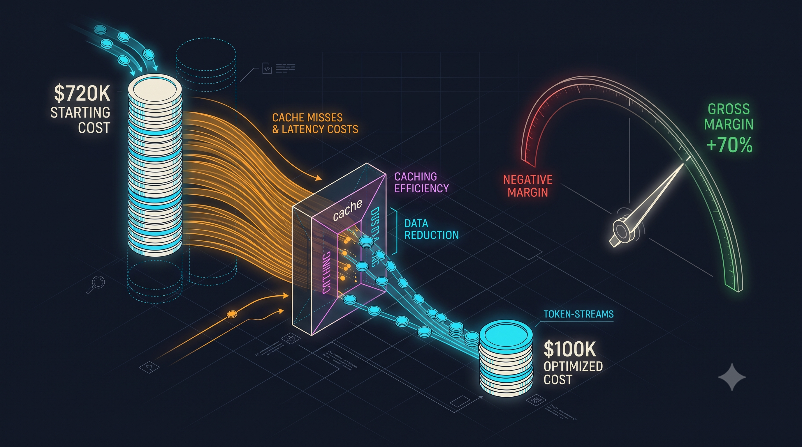
At 100K turns/day, input alone is 80K × 100K × 30 = 240B tokens/month × $3/M = $720K/month. That single number is why this is an engineering discipline.
Now apply prompt caching. Anthropic cache reads cost 10% of base input (a 90% discount → $0.30/M on Sonnet). Cache writes carry a premium: 1.25× base for the 5-minute TTL, 2× for the 1-hour TTL — so the first request on a fresh prefix costs more, and break-even arrives at the second hit. With 80% of input as stable cache-hit prefix:
$720K/month collapses toward ~$200K from caching alone, and with deferral + compaction (Sections 04.2, 04.5) realistically under $100K. The engineering below is worth on the order of $600K/month for a mid-sized platform — a full senior team, funded by the savings, several times over.
The existential framing is gross margin:
Charge $0.30/turn. Well-managed, , so . Un-managed — no caching, 20 tools every turn, RAG re-injected, history uncompacted — passes $0.30 and margin goes negative. The failure is usage-correlated and therefore adversarial: your most engaged power users (most tools, longest sessions) are precisely the accounts that flip you underwater. You bleed fastest on the customers you least want to lose, and a naive per-seat price hides it until a heavy cohort scales.
One more number that reframes the whole build: at 2026 open-weight pricing, filling a 1M-token window once ranges from $0.14 (DeepSeek V4 Flash) to $3.00 (Sonnet 4.6) to $10.00 (Claude Fable-class) — a 71× spread for the identical input. That spread is the entire argument of Section 07: for some platforms, the highest-leverage context decision is which token you are paying for in the first place.
03 — Step 0: measurement and ground-truth reward
You cannot optimize what you don’t measure, and you cannot score a tool without a definition of “success.” Two instruments precede all eight strategies.
3.1 Per-turn token accounting
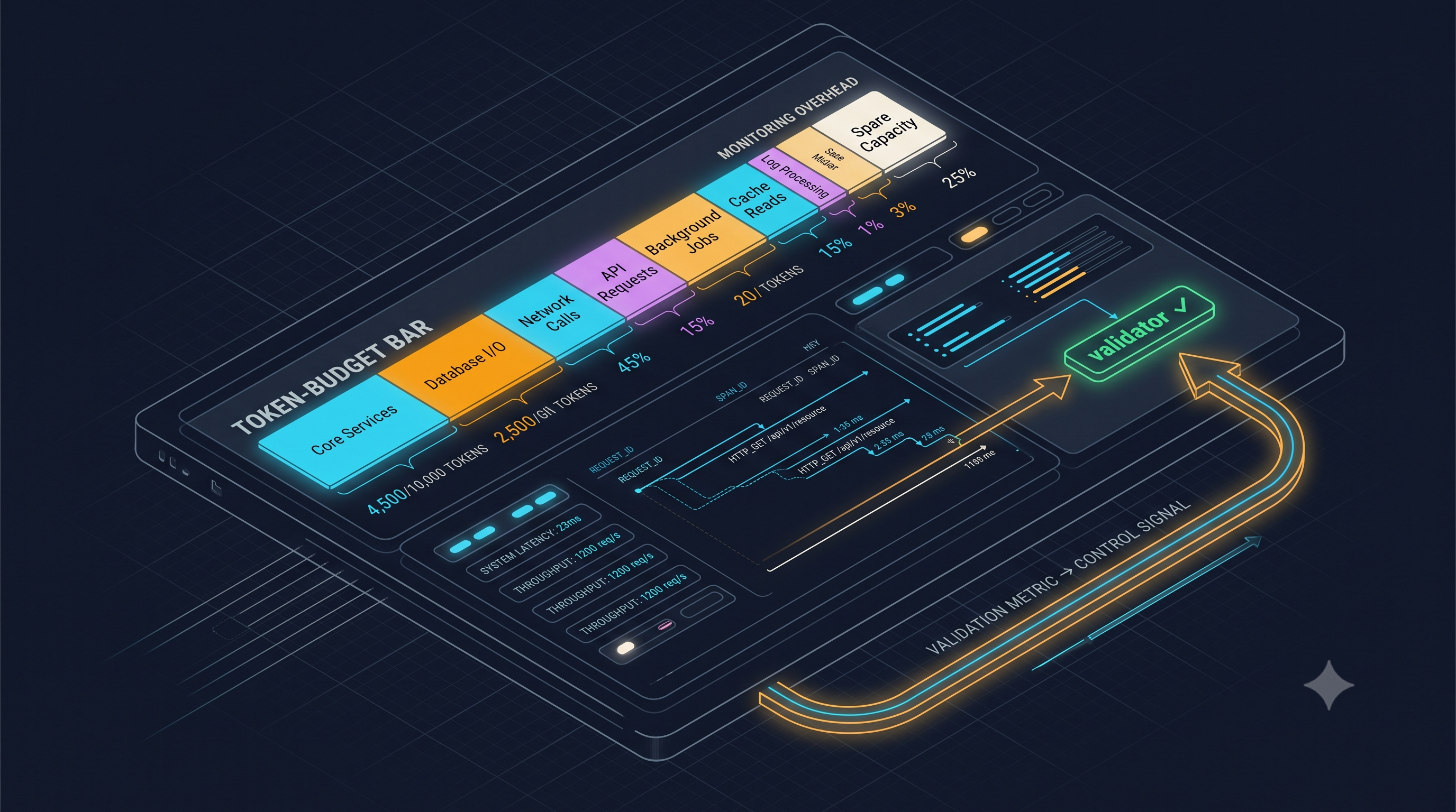
Every request logs a breakdown by component. This is the highest-ROI half-day in the guide because it tells you which term in to attack first — and the answer surprises most teams (usually tool descriptions or re-injected RAG, rarely raw history).
from dataclasses import dataclassimport tiktoken
@dataclassclass TokenBudget:    system: int = 0    agent_persona: int = 0    tool_descriptions: int = 0    memory_working_state: int = 0    history_verbatim: int = 0    history_summary: int = 0    retrieved_docs: int = 0    tool_results: int = 0    reasoning_scratch: int = 0
    @property    def total(self) -> int:        return sum(getattr(self, f) for f in self.__dataclass_fields__)
    def as_percentages(self, context_limit: int) -> dict[str, float]:        return {k: getattr(self, k) / context_limit                for k in self.__dataclass_fields__}
def account_turn(request_parts: dict, model: str = "gpt-4o") -> TokenBudget:    enc = tiktoken.encoding_for_model(model)    return TokenBudget(        system=len(enc.encode(request_parts["system"])),        agent_persona=len(enc.encode(request_parts.get("agent_persona", ""))),        tool_descriptions=sum(len(enc.encode(t))                              for t in request_parts.get("tools", [])),        memory_working_state=len(enc.encode(            request_parts.get("working_state", ""))),        history_verbatim=sum(len(enc.encode(m))                             for m in request_parts.get("history_verbatim", [])),        history_summary=len(enc.encode(            request_parts.get("history_summary", ""))),        retrieved_docs=sum(len(enc.encode(d))                           for d in request_parts.get("retrieved", [])),        tool_results=sum(len(enc.encode(r))                         for r in request_parts.get("tool_results", [])),        reasoning_scratch=len(enc.encode(            request_parts.get("reasoning", ""))),    )
Two notes. tiktoken with a GPT encoding is an approximation for Claude; the Opus 4.7+ tokenizer emits ~30% more tokens for the same text than earlier models, so for billing-grade numbers use the provider’s count_tokens endpoint and reserve tiktoken for relative attribution (which component is bloated). Second, emit this as structured telemetry mapped onto OpenTelemetry GenAI semantic conventions (gen_ai.usage.input_tokens, gen_ai.usage.output_tokens, and the operation/agent attributes) so cost flows into the same observability stack as latency and errors, sliceable by user, agent, and tool. Token accounting that isn’t queryable per-tenant is a log line, not an instrument.
3.2 Ground-truth reward (prerequisite for Strategy 8)
Before you can score tools or auto-tune context, define success. Four sources, ranked by fidelity:
- Downstream validator — an objective check verifies the output: SQL returned rows, code compiled, API returned 200, JSON validated against schema. Highest signal; use wherever it exists.
- Task completion — the overall task closed (user marked done, PR merged, ticket resolved).
- Explicit user feedback — thumbs up/down.
- LLM-as-judge — a second-pass model scores the trajectory. Lowest signal; fallback only, never the sole reward for anything touching money.
Compose reward with the token log so every scoring event carries its own cost and outcome — this is the join key the entire self-tuning loop depends on:
from dataclasses import dataclass, fieldfrom typing import Optional, Literalimport time
@dataclassclass RewardSignal:    task_type: str    tool_name: Optional[str]    success: bool    source: Literal["validator", "task", "feedback", "judge"]    confidence: float           # 1.0 for validators, lower for judge    timestamp: float = field(default_factory=time.time)
@dataclassclass TurnRecord:    session_id: str    turn: int    budget: TokenBudget    rewards: list[RewardSignal] = field(default_factory=list)
    def cost_usd(self, in_rate=3.0e-6, out_rate=15.0e-6, output_tokens=0):        return self.budget.total * in_rate + output_tokens * out_rate
Get the reward right first: every loop in Strategy 8 inherits its blind spots, and a bandit optimizing a bad reward will confidently converge on the wrong tools.
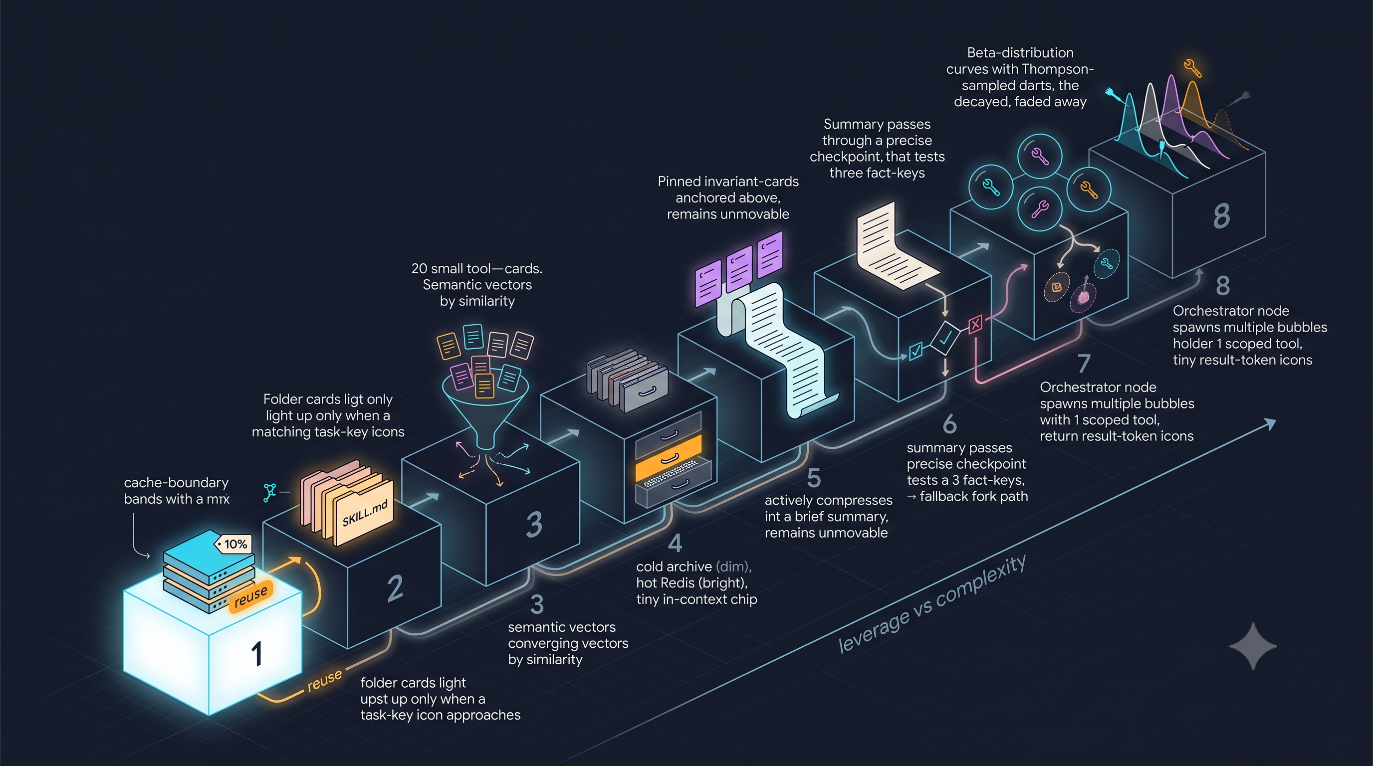
04 — The eight strategies
Ordered by leverage-per-complexity: lowest effort and highest impact first. The week estimates below are calendar weeks for one senior engineer, assuming the platform already has a working agent loop and CI; they are planning aids, not contracts, and they scale down with a second engineer and up with a hostile legacy codebase. Treat them as relative ordering signal, not absolute promises.
Strategy 1 — Prompt caching (do first)
Mark stable prefixes cacheable and stop re-encoding them every turn. Anthropic’s caching is explicit: attach cache_control: {"type": "ephemeral"} to a content block and everything from the request start up to that marker is cached. You get up to four breakpoints per request, which maps exactly onto the four stable boundaries of a Multi-Agentic Platform prompt, ordered most-stable to least-stable because the cache is a prefix cache (a one-token change invalidates everything after it):
- base system prompt (changes ~never),
- loaded tool descriptions (changes on onboarding),
- active agent persona (changes per active agent),
- retrieved documents (changes per retrieval).
Cache-aware cost per turn:
At 80% hit rate the input multiplier is — a 3.6× reduction with zero UX change.
import anthropicclient = anthropic.Anthropic()
def build_cached_request(system_prompt, tool_defs, persona, documents,                         history, user_message):    return dict(        model="claude-sonnet-4-6",        max_tokens=2048,        system=[            {"type": "text", "text": system_prompt,             "cache_control": {"type": "ephemeral", "ttl": "1h"}},  # boundary 1            {"type": "text", "text": tool_defs,             "cache_control": {"type": "ephemeral", "ttl": "1h"}},  # boundary 2            {"type": "text", "text": persona,             "cache_control": {"type": "ephemeral"}},               # boundary 3            {"type": "text", "text": documents,             "cache_control": {"type": "ephemeral"}},               # boundary 4        ],        messages=[*history, {"role": "user", "content": user_message}],    )
resp = client.messages.create(**build_cached_request(...))assert resp.usage.cache_read_input_tokens > 0   # health metric, not optional
Three production gotchas that each cost real money. (1) Cache writes are not free — 1.25× base for 5-minute TTL, 2× for 1-hour — so caching pays only when a prefix is reused within its TTL, which for an active session it always is; break-even is the second hit. (2) In March 2026 Anthropic silently changed the default TTL from 1 hour back to 5 minutes; a documented analysis of 119,866 Claude Code calls found this drove a 20–32% increase in cache-creation cost for long sessions, because any pause over five minutes expires the whole prefix and re-writes it at the 1.25× rate. For long-horizon agents set "ttl": "1h" explicitly and treat cache_read_input_tokens > 0 as a first-class per-turn health metric. (3) There is a minimum cacheable prefix (≈1K–4K tokens depending on model; 4,096 for the Opus 4.x / Haiku 4.5 / Sonnet 4.5 family) — prefixes below it silently do not cache, so short system prompts get no benefit and you should stop trying to cache them.
A subtlety most teams miss: any dynamic content injected into the cached prefix destroys the cache. A timestamp, a per-request session ID, or a “current date” string spliced into the system prompt means the prefix is never byte-identical across calls and your hit rate is zero. Move all volatile content to the user turn or behind the last cache boundary.
Complexity: ~2 engineering days. Do first. It captures 60–80% of total available savings before you touch anything else, which is exactly why starting anywhere else is a mistake.
Strategy 2 — Tool loading: defer + top-k retrieval per turn (do second)
The instinct on a tool-heavy platform is to shorten tool descriptions. Wrong lever. Don’t shorten them; defer them. Load only tool names and one-line summaries upfront (the “catalog”); retrieve full schemas on demand, either via a describe_tool(name) meta-tool the model can call, or — far better — by injecting the top-k most relevant tools per turn based on the current user message.
This is not folklore; it is the single best-measured result in the space. RAG-MCP (Gan & Sun, arXiv:2505.03275, May 2025) ran an MCP stress test scaling the tool pool from 1 to 11,100 servers and showed that semantic retrieval over a tool index — injecting only the selected descriptions — cut prompt tokens by more than 50% and more than tripled tool-selection accuracy, 43.13% vs 13.62% for the naive “all tools in context” baseline. The mechanism directly attacks two problems at once: token cost and decision fatigue (the model choosing wrongly among 20 schemas it barely attends to). For scale context, mcp.so listed 4,400+ MCP servers by April 2025; “load everything” was never going to survive.
Embed every tool description once at onboarding; embed the user message at turn start; retrieve top-k by cosine similarity; inject only those k full schemas. Twenty tools at 1.2K each is 24K; top-5 is ~6K — a 75% cut on the tool term per turn, with better selection accuracy as a bonus.
import numpy as npfrom dataclasses import dataclass
@dataclassclass Tool:    name: str    short_description: str  # <= 30 tokens, always in catalog    full_schema: str        # full JSON schema, injected only if selected    embedding: np.ndarray   # computed once at onboarding
class ToolRetriever:    def __init__(self, tools: list[Tool], k: int = 5):        self.tools = tools        self.k = k        self.embeddings = np.stack([t.embedding for t in tools])
    def top_k(self, query_embedding: np.ndarray) -> list[Tool]:        norms = np.linalg.norm(self.embeddings, axis=1)        qn = np.linalg.norm(query_embedding)        sims = (self.embeddings @ query_embedding) / (norms * qn + 1e-8)        return [self.tools[i] for i in np.argsort(-sims)[:self.k]]
    def format_catalog(self) -> str:        return "\n".join(f"- {t.name}: {t.short_description}" for t in self.tools)
    def format_top_k(self, query_embedding: np.ndarray) -> str:        return "\n\n".join(t.full_schema for t in self.top_k(query_embedding))
The catalog is stable, so it sits behind a cache boundary (Strategy 1); only the top-k block changes per turn, so it goes after the cached boundary. Enforcing a max description length at onboarding is worthwhile hygiene, but understand it as hygiene, not the lever — the win is deferral + top-k retrieval, not shorter text. Note RAG-MCP’s honest limitation, which you will hit: retrieval precision itself degrades as the registry grows into the thousands, which is exactly the motivation for Strategy 8 (learn which retrieved candidates actually succeed) layered on top of pure semantic retrieval.
Complexity: ~1 week. Do second. Savings on tool-heavy platforms: 70–90% of tool overhead.
Strategy 3 — Skills / conditional context (do third)
Skills generalize deferral from tools to instructions. A skill is an external SKILL.md — front-matter description plus a body — loaded only when the model detects a relevant task. Claude Code ships skills for docx, pptx, xlsx, and PDF that inject only when the corresponding task appears; Cursor’s .cursorrules and path-scoped rules load per-project. For a Multi-Agentic Platform, define a skill catalog per active domain (finance, engineering, sales) and route which SKILL.md files inject per turn.
---name: sql-analyticsdescription: Use when the user asks to query, aggregate, or analyze warehouse/tabular data. Triggers: "query", "how many", "trend", table names.---# SQL Analytics Skill- Prefer CTEs over nested subqueries.- Always LIMIT exploratory queries to 100 rows.- Validate column names against the schema catalog before emitting SQL.The router starts as keyword matching over the description front-matter and graduates to embedding similarity (reuse the Strategy 2 machinery). One production detail learned from Claude Code’s implementation: skills are re-injected after compaction, but large skills are truncated to a per-skill cap and the oldest-invoked skills are dropped once a total budget is exceeded — and truncation keeps the start of the file. So put the load-bearing instructions at the top of each SKILL.md; anything below the fold is best-effort.
Complexity: ~1 week. Do third. Best fit for multi-domain platforms.
Strategy 4 — Tiered memory (do fourth)
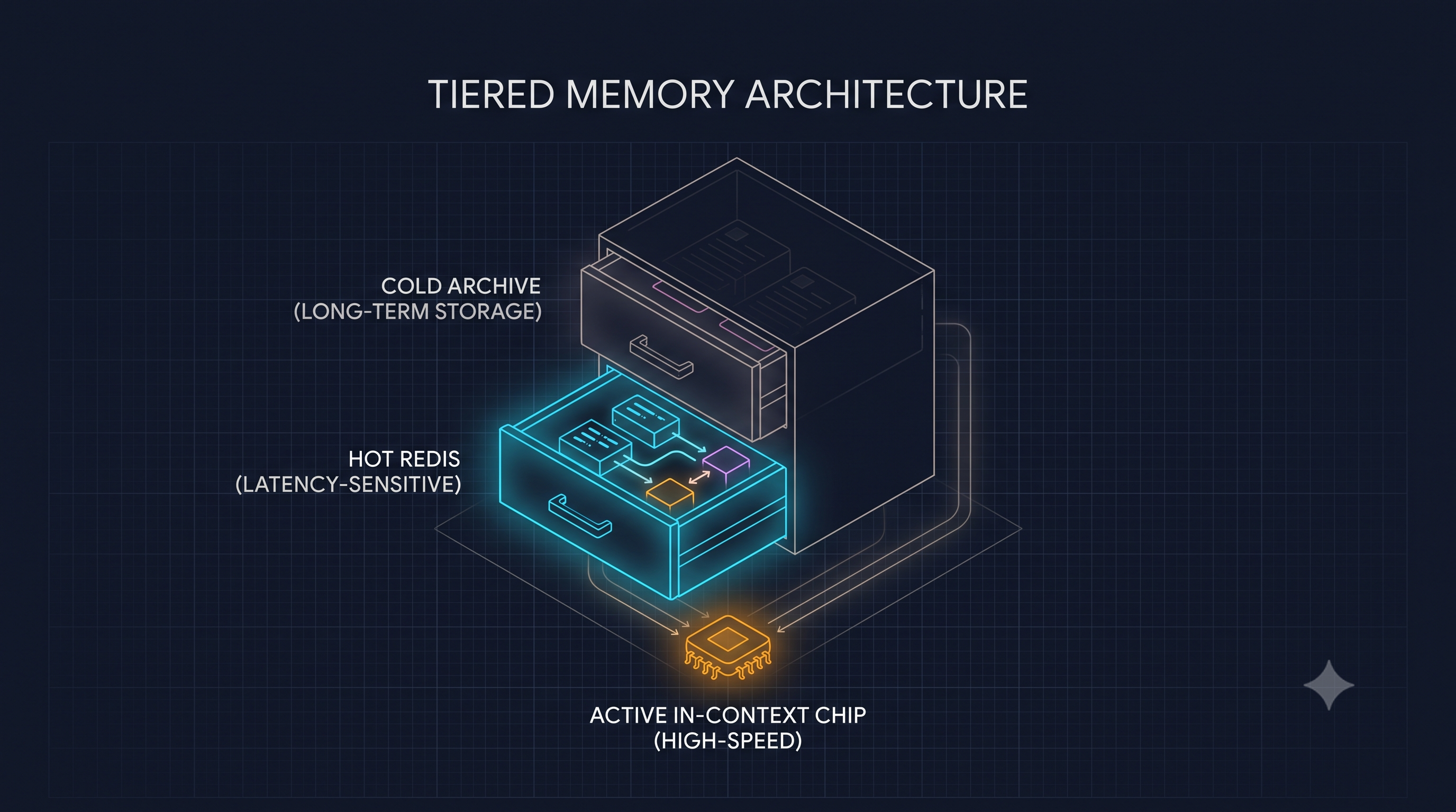
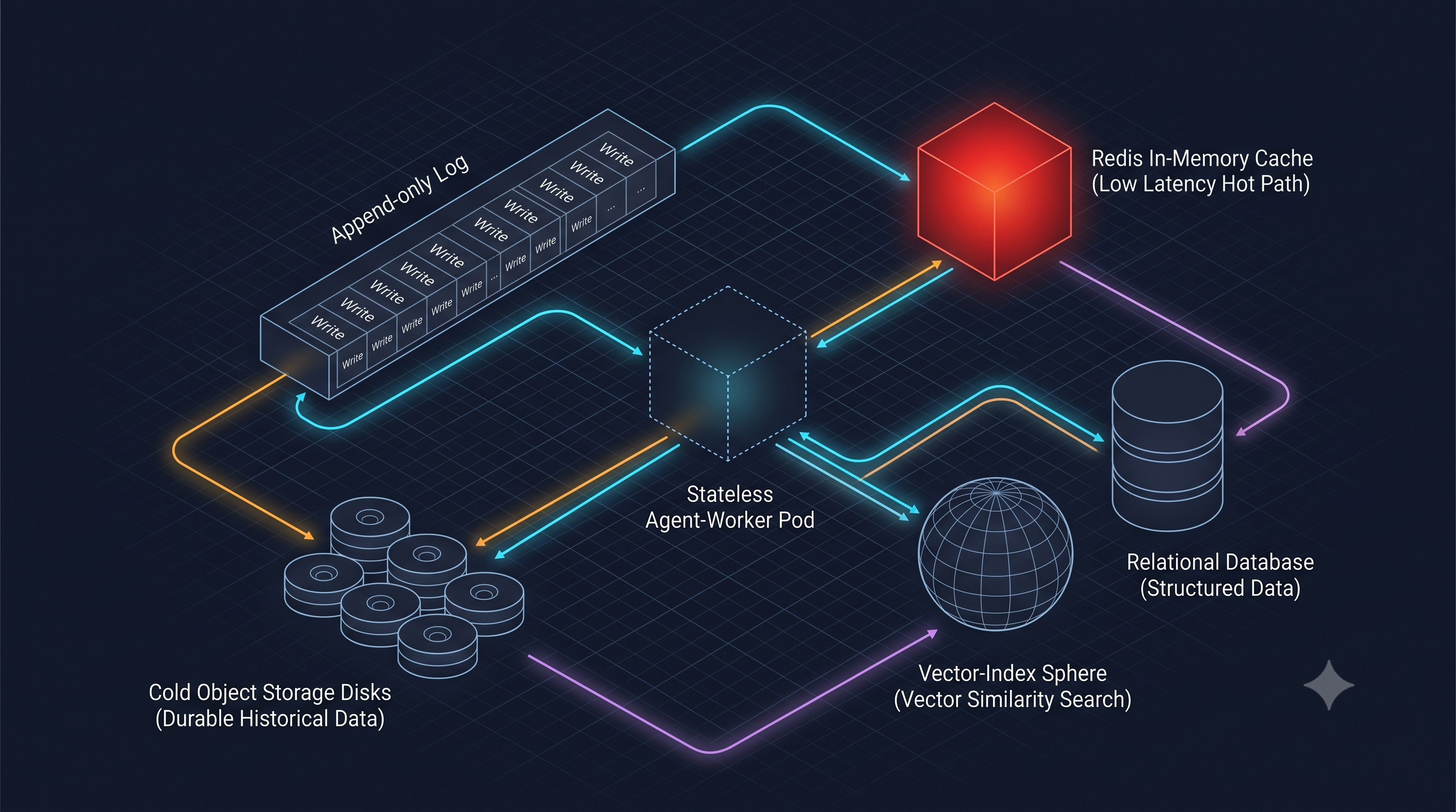
This is the strategy most platforms get wrong, because they inject memory as a raw free-text blob and watch quality decay as it grows. Split memory into three tiers with different residency rules:
- Tier A — Append-only log (never in context). Every turn, tool call, and reward is written to durable storage for audit, debugging, and replay. Never injected. This is the source of truth and the input to every offline job (Section 06 covers where it physically lives).
- Tier B — Typed working state (always in context, tiny). A structured object holding invariants the model must not forget: goals, constraints, entity IDs, prior decisions. Under ~500 tokens. Updated per turn as typed fields, never as free text.
- Tier C — Durable cross-session memory (loaded selectively). Session-crossing facts about the user — preferences, past outcomes — loaded only at session start or on semantic relevance, capped at ~1K tokens via vector retrieval.
Cap every memory artifact at ~200 lines. This is not a style preference; it is Lost in the Middle applied to your own files. A 600-line memory file buries its own middle third where attention is weakest.
The three-tier split is the production form of MemGPT (Packer et al., 2023, arXiv:2310.08560), which framed context as OS-style hierarchical memory with explicit paging between a small in-context tier and large out-of-context tiers — and which now ships as the Letta framework. But the more important 2025–2026 evidence is quantitative. Mem0 (Chhikara et al., ECAI 2025, arXiv:2504.19413) benchmarked selective memory against stuffing the full conversation into context on LOCOMO and reported 91% lower p95 latency (1.44s vs 17.12s), ~90% lower token cost, and a 26-point relative accuracy gain over a full-context/OpenAI-memory baseline (66.9% vs 52.9%). Its 2026 token-efficient algorithm reports ~91–92 on LoCoMo and ~93–94 on LongMemEval while averaging under 7,000 tokens per retrieval, versus 25,000+ for full-context. The lesson is blunt: dumping history into a big window is both slower and less accurate than retrieving a small, well-chosen memory. A-Mem (Xu et al., 2025) pushes further, representing memories as interconnected Zettelkasten-style notes with LLM-generated links that evolve as new facts arrive — useful when your platform needs multi-hop recall across sessions rather than flat lookup. And LongMemEval (Wu et al., ICLR 2025) quantifies the stakes of getting this wrong: commercial assistants show roughly a 30-point accuracy drop versus oracle retrieval, almost all of it recoverable by better memory selection.
import jsonfrom pydantic import BaseModel, Fieldfrom datetime import datetime
class Decision(BaseModel):    turn: int    decision: str    rationale: str
class WorkingState(BaseModel):    """The typed state the model always sees. Cap ~500 tokens."""    session_id: str    active_agent: str    goals: list[str] = Field(default_factory=list, max_length=5)    constraints: list[str] = Field(default_factory=list, max_length=5)    entity_ids: dict[str, str] = Field(default_factory=dict)   # role -> id    decisions: list[Decision] = Field(default_factory=list, max_length=10)    last_updated: datetime
    def to_prompt_section(self) -> str:        parts = ["## Working state\n"]        if self.goals:       parts.append("Goals: " + "; ".join(self.goals))        if self.constraints: parts.append("Constraints: " + "; ".join(self.constraints))        if self.entity_ids:  parts.append("IDs: " + ", ".join(f"{k}={v}" for k, v in self.entity_ids.items()))        if self.decisions:            parts.append("Prior decisions:")            for d in self.decisions[-5:]:                parts.append(f"  - T{d.turn}: {d.decision}")        return "\n".join(parts)
class AppendOnlyLog:    """Never in context. Durable audit trail."""    def __init__(self, sink):   # sink = Kafka topic, Postgres table, S3 writer        self.sink = sink    def append(self, event: dict) -> None:        event["timestamp"] = datetime.utcnow().isoformat()        self.sink.write(json.dumps(event) + "\n")
The typed constraint is the whole trick: because WorkingState is a bounded Pydantic model, it cannot silently grow to 5K tokens the way a free-text memory string does. The type system enforces the token budget mechanically, which is the only enforcement that survives contact with production.
Complexity: ~2 weeks. Do fourth. Impact: unlocks long-horizon agents that don’t degrade as sessions extend.
Strategy 5 — Anchored compaction with pinned invariants (do fifth)
Rolling summarization alone is dangerous. Summaries drift; worse, the model begins trusting a lossy compression of ground truth, and once a constraint falls out of the summary it is gone with no signal of its absence. Anchor the compaction: pin the invariants (goal, constraints, IDs, final decisions) in a section that is never compressed, and re-read those pinned facts from durable storage after compaction — not from the already-drifting context.
Algorithm: (1) at >50% utilization, initiate compaction; (2) keep the last N turns verbatim (N=3); (3) summarize turns older than N; (4) emit the pinned-invariants section read from disk; (5) concatenate pinned + summary + last_N.
from typing import Callable
def anchored_compact(history, pinned: WorkingState, keep_verbatim=3,                     summarizer: Callable = ...):    if len(history) <= keep_verbatim:        return history    to_summarize, verbatim = history[:-keep_verbatim], history[-keep_verbatim:]    summary = summarizer(to_summarize)    pinned_section = pinned.to_prompt_section()   # from durable storage — anti-drift    return [        Message(role="system", content=pinned_section),        Message(role="system", content=f"## Prior turn summary\n{summary}"),        *verbatim,    ]
Anthropic now ships this as a server-side primitive, which is the strongest possible endorsement of the pattern: the Messages API offers server-side compaction (beta header compact-2026-01-12, strategy compact_20260112 under context_management.edits). It detects when input tokens cross a configurable trigger, generates a <summary> block, drops all prior blocks, and continues from the summary; instructions lets you steer what to preserve (“keep code snippets, variable names, technical decisions”) and pause_after_compaction lets you meter cumulative usage against a budget. There is also a lighter context-editing strategy that simply clears stale tool results from agentic workflows without full summarization — the cheapest possible compaction, ideal when your bloat is old tool_result blocks rather than reasoning.
resp = client.beta.messages.create( betas=["compact-2026-01-12"], model="claude-opus-4-8", max_tokens=4096, messages=messages, context_management={"edits": [{ "type": "compact_20260112", "trigger": {"type": "input_tokens", "value": 150000}, "instructions": "Preserve entity IDs, constraints, and final decisions verbatim.", }]},)Trigger at 50% utilization, not 90%. Claude Code’s evolution is the case study: it reserves a fixed ~33K-token compaction buffer (down from 45K) and auto-compacts around ~83.5% of the window, and the field-tested finding from practitioners is that sessions stopping near 75% utilization ship higher-quality code than sessions run to 90%, because the extra working memory preserves reasoning. Compacting early also preserves cache state, since compaction rewrites a prefix the cache can re-warm. Even with server-side compaction available, keep the pinned-from-disk step: the server summary is still a summary, and re-reading invariants from durable storage is your only guarantee against silent constraint loss.
Complexity: ~1 week. Do fifth. Impact: sustains long conversations without quality cliffs.
Strategy 6 — Externalization + golden-fact verification (do sixth)
Large tool outputs — SQL result sets, API responses, documents — should be written to files, referenced by path, and retrieved on demand. Do not summarize them in place. In-place summarization is lossy and irreversible: replace a 47-row result set with “returned some customer rows” and the rows are unrecoverable, and you won’t discover the loss until three turns later when the model invents a row count with total confidence.
The defense is the golden-fact eval. Before compacting or summarizing anything, extract a small set of verifiable statements (“customer ID is 12345”, “query returned 47 rows”, “deadline is 2026-08-15”), then programmatically test whether the summary can still answer them. Fail even one → expand the window or fall back to raw content.
import jsonfrom dataclasses import dataclassfrom typing import Callable, Literal
@dataclassclass GoldenFact:    question: str    expected_answer: str    tolerance: Literal["exact", "semantic"] = "exact"
def extract_golden_facts(content: str, llm: Callable) -> list[GoldenFact]:    prompt = ("Extract 3-5 verifiable specific facts from the content below. "              "For each, give a question it answers and the expected answer. "              f"Return JSON list of {{question, expected_answer}}.\n\nContent:\n{content}")    return [GoldenFact(**f) for f in json.loads(llm(prompt))]
def verify_summary(summary, facts, llm) -> tuple[bool, list[str]]:    failures = []    for f in facts:        ans = llm(f"Given this summary:\n{summary}\n\nAnswer: {f.question}\n"                  "Answer only with the fact.").strip()        if f.tolerance == "exact" and ans != f.expected_answer:            failures.append(f"{f.question}: got {ans!r}, expected {f.expected_answer!r}")        elif f.tolerance == "semantic" and not semantic_match(ans, f.expected_answer):            failures.append(f"{f.question}: semantic mismatch")    return not failures, failures
def safe_summarize(content, summarizer, llm, max_retries=2) -> str:    facts = extract_golden_facts(content, llm)    for attempt in range(max_retries):        summary = summarizer(content, target_ratio=0.3 - attempt * 0.1)        ok, failures = verify_summary(summary, facts, llm)        if ok:            return summary        log.warning("summary failed golden-fact check: %s", failures)    return content  # fallback: keep raw content
The overhead is real (extraction + verification per summarization), but the alternative is silent context corruption, the single hardest production bug class to diagnose because there is no error, no stack trace — just a slow quality decline nobody can reproduce. This is also where learned compression earns deployment: LLMLingua / LongLLMLingua (Jiang et al., 2023, arXiv:2310.05736, 2310.06839) reach ~20× compression at under 2% quality loss using a small model, and RECOMP (Xu et al., 2023, arXiv:2310.04408) trains a compressor specifically for RAG contexts that beats zero-shot LLM summarization. Both remain underused in production precisely because teams fear silent loss; golden-fact verification is the guardrail that makes them safe to turn on.
Complexity: ~2 weeks. Do sixth. Impact: prevents the silent-degradation bugs that are hardest to debug.
Strategy 7 — Subagent isolation per MCP with explicit tool scoping (do seventh)
For platforms coordinating multiple team-owned MCPs, spawn a worker subagent per MCP with its own isolated context. The subagent sees only its scoped MCP’s tools plus the delegated sub-task, does the work, and returns a compact structured summary — typically under 500 tokens — to the orchestrator, whose window never sees the subagent’s turn-by-turn reasoning.
Scope tools explicitly. Do not assume inheritance. If the orchestrator holds tools A, B, C and delegates a task needing C, the subagent gets only C plus a control tool like return_result. This prevents cross-MCP contamination and keeps the subagent’s own context small.
from dataclasses import dataclassfrom pydantic import BaseModel
@dataclassclass SubagentSpec:    task: str                       # what to do    scoped_tools: list[str]         # explicit names, NOT inherited    mcp_context: str                # which MCP this subagent serves    max_turns: int = 10    result_schema: type[BaseModel]  # shape to return
class Orchestrator:    def spawn_subagent(self, spec: SubagentSpec) -> BaseModel:        prompt = self._build_subagent_prompt(spec)   # fresh context, no parent history        result = run_agent_loop(            prompt=prompt,            tools=[self.tool_registry[t] for t in spec.scoped_tools],            max_turns=spec.max_turns,        )        return spec.result_schema.model_validate_json(result)
This is exactly Claude Code’s Task tool: a subagent runs in a clean window and returns a summary, keeping large file reads out of the parent context. Cursor’s Agent/Composer mode uses similar delegation for large refactors. It is also where reasoning-heavy work belongs: a subagent can burn 40K extended-thinking tokens in isolation and hand back a 300-token answer, keeping out of the orchestrator entirely.
There is a real systems cost worth flagging, because it becomes the bottleneck at scale and connects directly to Section 05: subagents fragment the KV cache. Each fresh subagent context is a cache miss on the shared prefix, and prefix-cache reuse across many short-lived agents is an open research problem — KVFlow (arXiv:2507.07400, 2025) shows a workflow-aware KV-cache scheduler beating SGLang’s hierarchical radix cache by up to 1.83× on multi-agent workloads specifically because naive LRU eviction and prefix fragmentation hurt agent trees. If you self-host (Section 07), your subagent design and your serving-layer cache policy are the same decision.
Complexity: ~3 weeks. Do seventh. Impact: multi-MCP coordination without context explosion.
Strategy 8 — Bandit scoring for tool selection (do last)
The most powerful strategy, and the one most often built first for the wrong reason (it’s the most fun). Replace hardcoded top-k with a Bayesian bandit that scores each tool by historical success, conditioned on task type. Successes rise, failures decay, new tools get explored automatically.
Foundation. For each (task_type, tool) pair, maintain a Beta distribution over success probability. Beta is the conjugate prior for the Bernoulli likelihood, so posterior updates are trivial addition:
with uniform. Time decay keeps recent outcomes weighted above ancient ones:
Thompson sampling gives Bayesian-optimal exploration: sample for each tool and pick the argmax of the samples, so wide (uncertain) posteriors occasionally sample high and get tried:
import numpy as npfrom dataclasses import dataclassfrom collections import defaultdict
@dataclassclass BetaBandit:    alpha: float = 1.0    beta: float = 1.0    last_updated: float = 0.0
    def decay(self, now, lam_per_day=0.99):        days = (now - self.last_updated) / 86400        factor = lam_per_day ** days        self.alpha = 1.0 + (self.alpha - 1.0) * factor   # decay toward prior        self.beta  = 1.0 + (self.beta  - 1.0) * factor        self.last_updated = now
    def update(self, success: bool, now: float):        self.decay(now)        self.alpha += 1 if success else 0        self.beta  += 0 if success else 1        self.last_updated = now
    def sample(self, rng): return rng.beta(self.alpha, self.beta)    def mean(self):        return self.alpha / (self.alpha + self.beta)    def uncertainty(self):        a, b = self.alpha, self.beta        return np.sqrt((a * b) / ((a + b) ** 2 * (a + b + 1)))
class ToolBandit:    def __init__(self, tools):        self.scores = defaultdict(lambda: defaultdict(BetaBandit))        self.tools = {t.name: t for t in tools}        self.rng = np.random.default_rng()
    def record(self, task_type, tool_name, success, now):        self.scores[task_type][tool_name].update(success, now)
    def select_top_k(self, task_type, candidate_tools, k):        samples = {n: self.scores[task_type][n].sample(self.rng) for n in candidate_tools}        return sorted(samples, key=samples.get, reverse=True)[:k]
Compose with Strategy 2, don’t replace it. Two passes: semantic retrieval narrows ~20 tools to ~15 candidates; Thompson sampling on those 15, conditioned on task type, picks the final top-5; only those 5 schemas enter context. Semantic relevance answers “which tools could apply”; the bandit answers “which have actually worked for this kind of task.” This is precisely the gap RAG-MCP flagged — retrieval precision decaying at thousands of tools — closed with a learned performance signal. Run a nightly scheduler: decay all Beta distributions to a canonical timestamp, recompute aggregate memory summaries, prune tools whose 95% posterior CI sits below 0.2 success, and emit per-task-type performance dashboards. Thompson-sampling-for-tool-use is an active 2024–2026 research thread (NeurIPS/ICML workshops); cite the current best at publish time.
Complexity: 3+ weeks. Do last. Impact: a self-tuning platform.
05 — Latency: the second bill, paid in milliseconds
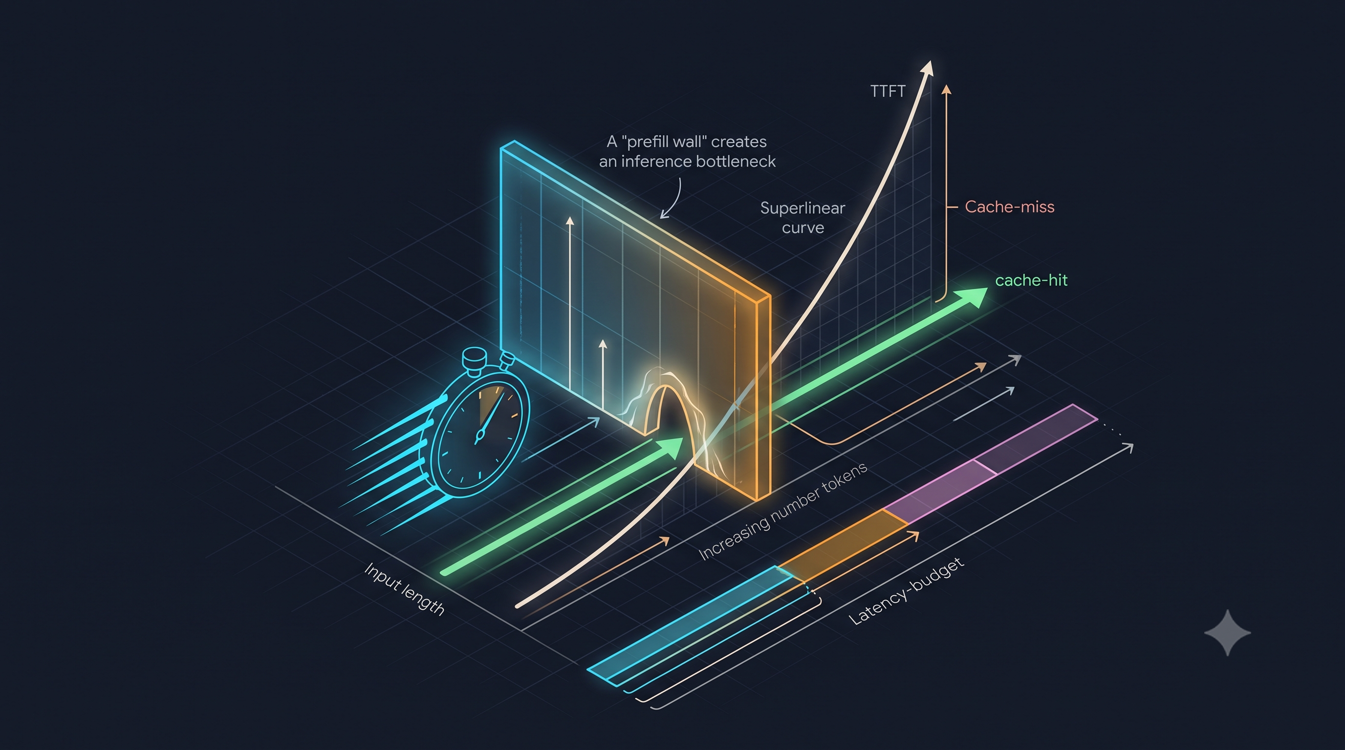
Cost is the invoice you see monthly; latency is the invoice your users see every turn, and on an agentic platform it is dominated by the same variable — input tokens. Understanding why connects context management directly to response time.
The prefill wall. Transformer self-attention is quadratic in sequence length, so time-to-first-token (TTFT) grows superlinearly with input size. An 87K-token prefill is not 10× an 8K prefill; it is worse, because the attention computation over the prefix must complete before the first output token streams. This is the single most important latency fact for agentic platforms: the same 87K of scaffolding that costs $0.24 also adds hundreds of milliseconds to seconds of TTFT before the user sees anything. Every strategy that shrinks the prefix — caching, deferral, compaction — buys latency and cost simultaneously.
Prompt caching is a latency optimization first, a cost optimization second. A cache read skips the prefill compute for the cached prefix entirely; the KV state is loaded, not recomputed. On long stable prefixes this is the difference between a multi-second and a sub-second TTFT. This is why cache hit rate belongs on your latency dashboard, not just your cost dashboard — a TTL regression (the March 2026 event) shows up as a latency regression for long sessions before finance notices the cost.
A latency budget for the request pipeline. Section 08’s reference flow has serial and parallel stages; budget them explicitly. Representative targets for a well-built platform:
| Stage | Typical budget | Notes |
|---|---|---|
| Token accounting | ≤1 ms | Pure arithmetic; never on the hot path if async |
| Skill routing (keyword) | ≤5 ms | Embedding router adds one vector op |
| Tool retrieval (embed query + top-k) | 10–40 ms | One embed call + a cosine over a few thousand vectors |
| Memory retrieval (Tier C) | 20–80 ms | Vector DB p95; Mem0 reports ~1.4s p95 end-to-end vs 17s full-context |
| Context assembly | ≤5 ms | String building |
| LLM TTFT (cache hit) | 200–800 ms | Dominated by uncached suffix length |
| LLM TTFT (cache miss) | 1–5 s+ | Full prefill of the whole prefix |
The retrieval stages (tool + memory) are added latency you are spending to save prefill latency — and the trade is almost always positive, because a 40 ms retrieval that removes 30K tokens of prefill saves far more than 40 ms of prefill. Mem0’s benchmark makes this concrete: selective memory cut p95 latency from 17.12s to 1.44s — a 91% reduction — precisely because it stopped prefilling 25K+ tokens per query.
Parallelism is the subagent’s other payoff. Strategy 7 isolates context; it also parallelizes it. Independent subagents (per MCP) run concurrently, so three subagents at 2s each cost 2s wall-clock, not 6s — but only if your serving layer can admit them without cache thrash. This is where self-hosting choices (Section 07) and orchestration choices couple: continuous batching (Orca’s iteration-level scheduling, as implemented in vLLM) is what lets concurrent subagents share GPU efficiently, and prefix-cache-aware routing is what keeps their shared prefix warm.
The tail is the product. Optimize p95/p99, not the mean. A single uncached 200K-token turn in a session blows the tail even if the median is fast, and agentic sessions are bursty by nature (a pause > TTL, then a heavy turn). Explicitly set the 1-hour cache TTL on stable prefixes for long sessions specifically to flatten this tail; the cost is a 2× write premium paid once, and the return is that the heavy turn after a pause is a cache read (sub-second) rather than a cold prefill (multi-second).
06 — Memory storage infrastructure: where the three tiers actually live
The three memory tiers of Strategy 4 have three different physical homes, three different durability requirements, and three different failure modes. Getting this wrong is how a platform that manages tokens correctly still loses data — or pays a database bill that dwarfs its token bill. This is the section the model-focused write-ups skip, and it is pure production engineering.
The governing principle: match the store to the access pattern, and never put anything in the container filesystem that must survive the pod. Agent workers are stateless, horizontally scaled, and rescheduled constantly (autoscaling, spot reclamation, rolling deploys). A file written to a container’s local disk is gone the moment that pod dies, which for a spot-backed inference fleet may be minutes. Treat container-local storage as scratch only.
The tier-to-store mapping
| Tier | Access pattern | Store | Durability | Why |
|---|---|---|---|---|
| A — Append-only log | Write-heavy, sequential, rarely read online | Kafka / Kinesis → object storage (S3/GCS), or an append-only Postgres/ClickHouse table | Must never be lost | Audit, replay, offline bandit training. Cheap per-GB, write-optimized. |
| B — Typed working state | Read + write every turn, tiny, latency-critical | Redis (or Redis-compatible: Valkey, ElastiCache, MemoryStore) | Regenerable but hot | Sub-ms reads on the request hot path. This is the one thing you touch every turn. |
| C — Cross-session durable memory | Semantic read on session start / relevance | Vector DB (pgvector, Qdrant, Weaviate, Milvus) + a system-of-record row store | Must survive; can be re-embedded | Similarity search is the access pattern; a flat KV store can’t do it. |
Tier B — the hot path — belongs in Redis, not a file and not Postgres. Working state is read and written on every single turn, it is tiny (under 500 tokens ≈ a few KB serialized), and it is latency-critical (it sits before the LLM call). Redis gives you sub-millisecond reads, atomic updates (HSET/JSON.SET), and natural TTL for session expiry. Key by session: ws:{session_id}. Redis is regenerable — if you lose it you can replay Tier A to reconstruct working state — so you can run it as a cache tier without cross-region replication if budget matters, but size it for your concurrent-session count, not your total-user count.
Tier A — the log — belongs in an append-only, write-optimized sink, streamed off the box immediately. The AppendOnlyLog in Strategy 4 must write to a durable sink (a Kafka topic, a Kinesis stream, or directly to object storage via a buffered writer), not to open(path, "a") on the container. From there it lands in cheap columnar storage (S3 + Parquet, or ClickHouse) for the nightly bandit job and for audit. This is your compliance and debugging spine; it is also the training data for Strategy 8, so its schema is a first-class API, not an afterthought.
Tier C — durable memory — needs a vector index plus a row-store system of record. The vector DB answers “what past facts are relevant to this session,” but you keep the canonical text and metadata in a durable row store (Postgres) and treat the vector index as a derived, re-buildable artifact — because you will re-embed when you change embedding models, and you do not want your only copy of a user’s memory trapped in a vector index you can’t migrate. pgvector collapses both into one Postgres if your scale allows (single system, transactional, easy backup); dedicated stores (Qdrant, Milvus) win at very high vector counts or when you need advanced filtering and horizontal sharding.
The container question, answered directly
If you deploy on Kubernetes: agent worker pods should be stateless Deployments with no persistent volume — all state lives in the external stores above. You do not need a PersistentVolume for agent workers, and attaching one is an anti-pattern that breaks horizontal scaling and rescheduling. Reserve PersistentVolumes and StatefulSets for the stateful backing services you self-host — a self-managed Redis, Postgres, or Qdrant needs a PV (typically a cloud block volume: EBS, PD, Azure Disk) with a volumeClaimTemplate, stable network identity, and a backup policy. The decision rule is crisp: stateless compute (agent workers) = Deployment, no PV; stateful data (your databases) = StatefulSet, PV, backups — or, better for most teams, use managed services (ElastiCache, RDS/Cloud SQL, managed Qdrant) and let the provider own the PV, replication, and failover.
The one legitimate use of container-local disk is Strategy 6’s externalization scratch — large tool outputs written to a file and referenced by path within a single session’s lifetime. Even here, prefer a session-scoped object-storage prefix (s3://scratch/{session_id}/...) or a shared ephemeral volume (an emptyDir, or a RWX volume if multiple pods in a session must share) so a mid-session pod reschedule doesn’t lose the externalized artifact. If a tool output must outlive the session, it is Tier A/C data, not scratch.
What the KV cache is (and isn’t) in this picture
A frequent confusion: the model’s KV cache — the attention key/value tensors that prompt caching reuses — is not your memory tier. On a hosted API (Anthropic, OpenAI) the KV cache is the provider’s internal state; you influence it only through cache-control markers and prefix stability, and you never store or persist it. It lives for the TTL and vanishes. Your three memory tiers are application state you own in Redis/Postgres/object storage. The KV cache and your memory tiers interact — a stable Tier B rendering keeps the prefix byte-identical and therefore cache-friendly — but they are different layers with different owners. For a deep treatment of KV cache mechanics at the serving layer, see our KV cache engineering guide. This distinction becomes load-bearing the moment you self-host, where the KV cache becomes your problem too (next section).
07 — Self-hosted open models: how every strategy changes when you own the GPU
A user who picks an open-weight model (Llama 4, Qwen 3.x, DeepSeek V3/V4) — or a platform that offers self-hosted models as a tier — changes the economics and the mechanics of every strategy above. This is not a footnote; for high-volume platforms it can be the single largest context-related decision, because it changes which token you are paying for.
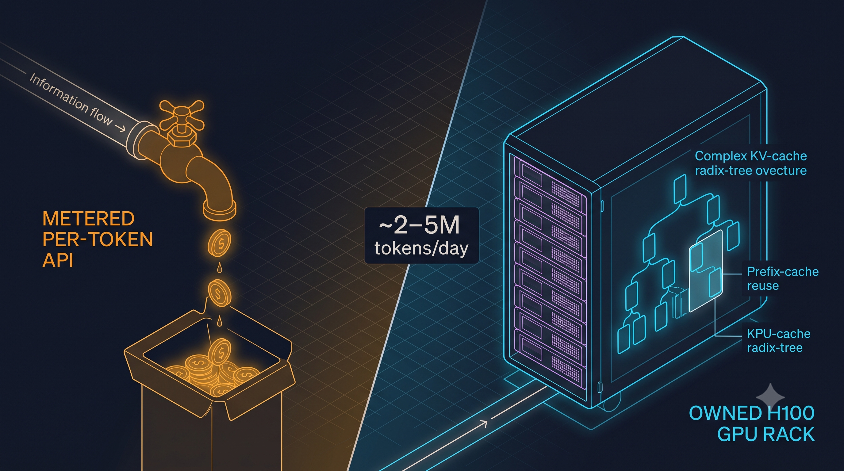
The economics flip: from per-token to per-GPU-hour
Hosted APIs bill per token; self-hosting converts that into a fixed GPU cost you amortize across all tokens. The crossover is well-characterized in 2026: self-hosting on reserved GPU capacity breaks even against frontier APIs at roughly 2M–5M tokens/day over a 12-month horizon. Below that, the API wins on both cost and operational simplicity; above it, owning the fleet wins, and the margin widens with volume. The context implication is profound: once you own the GPU, marginal input tokens are nearly free (they cost GPU-seconds, not dollars-per-million), so the cost pressure on context partially inverts — but the latency and quality pressures do not, because prefill is still quadratic and context rot is model-agnostic. You stop optimizing context to save dollars and start optimizing it to save GPU-seconds and preserve accuracy, which usually points the same direction.
Rough 2026 landscape for the self-host decision:
| Model | Params (total/active) | Context | Self-host footprint | License |
|---|---|---|---|---|
| Qwen3-32B (dense) | 32B | ~131K (YaRN-extended) | 1× H100 | Apache 2.0 |
| Llama 4 Scout (MoE) | 109B / 17B | 10M | 1× H100 (quantized) | Llama Community |
| Llama 4 Maverick (MoE) | 400B / 17B | 1M | multi-GPU | Llama Community |
| DeepSeek V3 (MoE) | 671B / 37B | ~128–160K | 8× H100 (FP16) | MIT |
Llama 4 Scout’s 10M window on a single H100 is genuinely novel and reframes some RAG workloads — but NoLiMa and context rot still apply: 10M advertised is not 10M effective, and filling it is quadratic-expensive in latency even when the token cost is amortized to near-zero. A 10M window is a reason to be less reckless about what you put in it, not more.
What breaks, and what you gain
Prompt caching (Strategy 1) becomes your problem — and your advantage. There is no cache_control: ephemeral API; instead, your serving engine’s automatic prefix caching does the equivalent, and you control the eviction policy directly. vLLM implements automatic prefix caching via block-level KV hashing (PagedAttention; Kwon et al., SOSP 2023, arXiv:2309.06180) and delivers 2–4× the throughput of naive HuggingFace serving. SGLang’s RadixAttention (Zheng et al., NeurIPS 2024, arXiv:2312.07104) organizes the KV cache in a radix tree for automatic prefix sharing with LRU eviction and, on prefix-heavy RAG and agentic workloads, reportedly leads vLLM by ~29% throughput on H100 (≈16.2K vs 12.5K tok/s) and up to 6× on the most prefix-repetitive pipelines. The advantage over the hosted API is control: you set the eviction policy, you can pin hot prefixes, and you can adopt workflow-aware schedulers — KVFlow (arXiv:2507.07400) for multi-agent trees, Mooncake (KVCache-centric disaggregated serving) and LMCache (arXiv:2510.09665) for cross-request KV reuse at enterprise scale, CacheBlend (arXiv:2405.16444) / RAGCache (arXiv:2404.12457) / TurboRAG (arXiv:2410.07590) for precomputing and fusing KV of RAG chunks. The disadvantage: all of this is now your on-call rotation.
The four cache boundaries become KV-block boundaries. The same discipline applies — stable prefix first, volatile content last — but now the mechanism is block-hash matching, and the same anti-pattern bites harder: any per-request dynamic content in the prefix busts the prefix-cache block and forces recompute. Structure the prompt so the system prompt, tool catalog, and persona occupy whole, stable KV blocks.
Subagents (Strategy 7) become a KV-cache scheduling problem, not just a context problem. On a hosted API the provider absorbs the fragmentation; self-hosted, spawning many short-lived subagent contexts fragments your radix tree and evicts hot prefixes under LRU. This is exactly what KVFlow and TokenCake (arXiv:2510.18586) address, and why a naive “spawn a subagent per tool call” design that is free on Anthropic can tank throughput on your own vLLM fleet. Budget subagents against KV-cache capacity, and prefer a workflow-aware cache policy if your agent trees are wide.
Tokenizer and effective-context differences ripple through everything. Each model family tokenizes differently, so your Strategy-3 token budgets and Strategy-5 compaction thresholds must be recomputed per model — a 200-line memory file is a different token count on Qwen than on Llama. And effective context varies by model independent of the advertised number (RULER/NoLiMa), so your 50%-utilization compaction trigger should be tuned to the effective length you measure, not the spec-sheet window.
The strategies that don’t change at all: tiered memory (Strategy 4), anchored compaction’s pinned-from-disk discipline (Strategy 5), golden-fact verification (Strategy 6), and bandit scoring (Strategy 8) are all application-layer and model-agnostic. They work identically whether the token was billed by Anthropic or computed on your H100. This is the reassuring part: most of the guide transfers unchanged, and only the caching/serving/subagent layer is model-host-specific.
A hybrid routing note
Most mature platforms in 2026 run hybrid: cheap open models (or Haiku-class) for routing, extraction, and classification; frontier models for the hard reasoning turns. Reported cost reductions from disciplined hybrid routing land in the 60–83% range. Context management is what makes hybrid routing safe — a well-compacted, well-scoped context is portable across models, so you can route the same assembled context to a $0.14/1M open model or a $3/1M frontier model based on task difficulty, and the bandit (Strategy 8) can learn the routing threshold per task type from the same reward signal it uses for tools.
08 — Case studies: how production systems actually do this
These are not logos on a slide. Each system below made specific, load-bearing context-management decisions you can copy.
Claude Code (Anthropic) — the most complete public reference implementation
Claude Code is the closest thing to a fully worked example of this entire guide shipping in production, and its mechanics are documented in detail worth studying.
Layered, tiered instruction loading. At session start it loads CLAUDE.md (project instructions, read every session — “free context that survives restarts,” but every token spent there is a token unavailable for conversation, so the guidance is keep it lean and prune it), auto-memory files, MCP tool names (not full schemas), and skill descriptions (not bodies). This is Strategies 2, 3, and 4 simultaneously: the tool catalog is lazy, skills are conditional, and CLAUDE.md is a form of pinned working state. /context gives a live per-category breakdown (“your memory files are eating 15% before you start — fix that”), and /memory shows which instruction files loaded.
Compaction, quantified. Claude Code reserves a fixed compaction buffer — ~33K tokens (reduced from 45K in early 2026) — and auto-compacts as you approach the limit (default trigger ≈83.5% of the window, tunable via CLAUDE_AUTOCOMPACT_PCT_OVERRIDE, with PreCompact/PostCompact hooks that run outside the context window). Compaction summarizes history into a continuation summary that preserves decisions, file paths, and patterns while dropping raw transcript. /compact "keep the API design and schema, summarize the debugging" steers preservation; /clear resets history entirely; /rewind steps back. The hard-won field lesson: stopping near 75% utilization ships higher-quality code than running to 90%, because working memory is reasoning capacity — the direct empirical basis for Strategy 5’s “compact at 50%, not 90%.” A crucial compaction subtlety they document: path-scoped rules and nested CLAUDE.md files loaded into message history get summarized away by compaction and reload only when a matching file is re-read, so anything that must survive compaction belongs in the root CLAUDE.md — the pinned tier. Skills are re-injected post-compaction but truncated to a per-skill cap (keeping the file’s start), with oldest-invoked skills dropped first.
Server-side compaction and context editing as API primitives. The same machinery is exposed on the Messages API (compact-2026-01-12 beta, context_management.edits) with configurable trigger, custom instructions, and pause_after_compaction for budget metering — plus lighter context editing that clears stale tool_result blocks without full summarization. Anthropic’s docs name the underlying phenomenon “context rot” and state the thesis of this guide outright: more context isn’t automatically better; curation matters as much as capacity.
Subagents and the memory tool. The Task tool spawns subagents with isolated windows that return only summaries (Strategy 7) — the docs explicitly advise “delegate large reads to a subagent so file contents stay in its window, not yours.” The memory tool provides a multi-session persistence pattern (Tier C). Skills for docx/pptx/xlsx/PDF are the canonical conditional-context example (Strategy 3). Net result: multi-hour autonomous sessions on 200K models, and 1M-context variants (Sonnet 4.6, Opus 4.6+) for when the window itself must be larger.
Cursor — retrieval as the primary context strategy
Cursor treats the codebase as a retrieval corpus rather than something to stuff into context. Codebase indexing embeds files and retrieves the relevant ones per query — Strategy 2 applied to code, at repo scale. @-mentions are explicit, user-driven context inclusion (the human overriding retrieval when they know better), and .cursorrules plus path-scoped rules are per-project conditional context (Strategy 3). Its modes are distinct context strategies with different budgets: Chat (tight, question-scoped context), Composer/Agent (broad, multi-file, delegating large refactors to agent-style workers that keep bulk file reads out of the primary thread). The lesson for a platform builder: expose retrieval, explicit inclusion, and conditional rules as three separate user-facing controls, because they serve different intents — automatic relevance, manual override, and standing policy.
Aider — anchored compaction via the repository itself
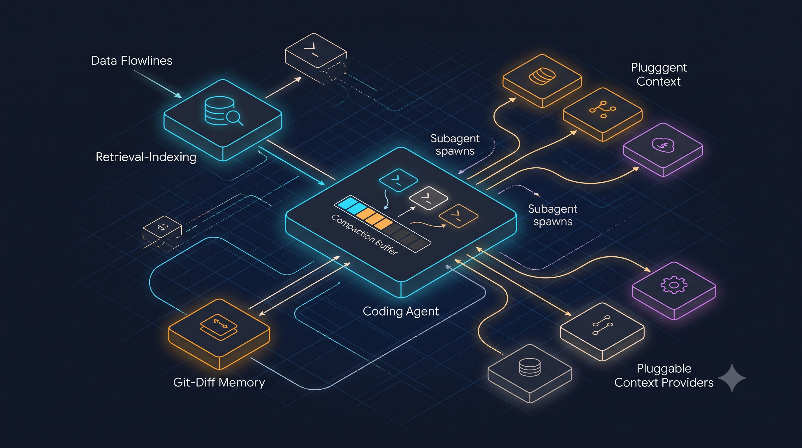
Aider’s repo-map and git-diff-aware context are anchored compaction in its purest form: the git diff is an always-current, ground-truth summary of what changed, so Aider never has to summarize file state lossily — it re-derives it from the repository, which is the disk-backed source of truth. This is the anti-drift discipline of Strategy 5 achieved structurally rather than with an LLM summarizer, and it is why Aider stays coherent on long editing sessions with a comparatively small context: it treats the repo as external memory and pulls only the diff and the relevant map into the window.
Windsurf and Continue — context providers as a first-class abstraction
Windsurf (Cascade) and Continue generalize the right architectural instinct: make each context source a pluggable, independently measurable provider. Continue exposes “context providers” explicitly — codebase, docs, terminal output, git, custom — so each source can be added, ranked, budgeted, and instrumented separately. For a Multi-Agentic Platform this is the pattern to copy at the architecture level: every term in should be a named provider with its own token budget and its own hit-rate metric, not an undifferentiated blob assembled ad hoc. When each provider is measurable, Section 03’s token accounting becomes trivial and Strategy 8’s optimization has clean signal.
Letta (MemGPT) and Mem0 — memory as a product, not a prompt
Letta productizes MemGPT’s OS-style paging between an in-context “main memory” and out-of-context archival memory, with the model itself issuing memory-management calls — the reference implementation of Strategy 4’s tiering. Mem0 productizes the retrieval side with the benchmark numbers that justify the whole approach (Section 04.4): selective memory at under 7K tokens/query beating full-context at 25K+ tokens on LoCoMo/LongMemEval, at 91% lower p95 latency. The takeaway is strategic: by 2026, “AI memory” is its own architectural component with its own benchmark suite (LoCoMo, LongMemEval, BEAM) and its own vendors — you can buy Tier C rather than build it, and the build-vs-buy line is now a real decision rather than a foregone “roll your own.”
A reference Multi-Agentic Platform — the full request flow
Assembling all eight strategies plus Sections 05–07, one turn flows:
user message → token accounting (§3.1, async, off hot path) → skill router selects SKILL.md files (§4.3) → tool retriever: semantic top-15 then bandit top-5 conditioned on task type (§4.2 + §4.8) → memory load: Tier B working state from Redis + Tier C relevant facts from vector DB (§4.4, §6) → context assembly behind four cache boundaries: system ‖ tool catalog+top-k schemas ‖ persona ‖ working-state+summary+verbatim-last-N (§4.1, §4.5) → LLM call (hosted with cache_control, or self-hosted with prefix caching) (§4.1, §7) → response + tool calls → per-MCP subagents spawned concurrently with scoped tools, returning ≤500-token structured results (§4.7, §5 parallelism) → large tool outputs externalized to session scratch with golden-fact-verified summaries (§4.6) → append-only log to Kafka→S3 (§6) → reward capture from downstream validators (§3.2) → nightly: bandit decay+update, memory consolidation, tool pruning (§4.8).
Every arrow is a strategy; every strategy is independently measured by the token log and the latency budget; every store is chosen by access pattern. That is the whole system.
09 — The MCP-specific problem
MCP tool descriptions follow a JSON schema (name, description, input_schema). A five-parameter tool with per-parameter descriptions and enums easily reaches 400–800 tokens; twenty is 8–16K of overhead before the user types a word — and Anthropic’s docs note the tool-use system prompt itself adds a few hundred tokens on top (~497 on Sonnet 4.6, higher on Opus). At ecosystem scale the problem is worse: mcp.so listed 4,400+ servers by April 2025, and RAG-MCP’s stress test ran to 11,100.
Recommendations, in priority order (the ordering is the point):
- Defer + top-k retrieval (Strategy 2) — the real lever, with RAG-MCP’s >50% token cut and 3× accuracy gain as the evidence. Load the catalog; inject only relevant full schemas.
- Compress at load time — strip examples and long parameter prose from the injected schema; expose the full version via
describe_tool. - Group related tools into packages loaded together, so retrieval operates on coherent bundles rather than fragmenting a workflow across separate hits.
- Cache tool descriptions aggressively (Strategy 1 / prefix caching) — they’re stable between onboarding events, so they belong on a 1-hour cache boundary or a pinned KV block.
- Per-MCP subagent isolation (Strategy 7) — contains the blast radius of one team’s badly-written 2K-token tool schema and prevents cross-MCP contamination.
- Enforce a max description length (~300 tokens) at onboarding — hygiene applied at the door, not the strategy.
The onboarding pipeline is where you enforce most of this: validate schema size, generate the short-description and embedding, and reject or auto-compress oversized descriptions before they ever reach a user’s context. Context hygiene is cheapest when applied at ingestion.

10 — The research foundation (2023–2026)
Organized by the problem each body of work solves, so you can go deeper on whichever term of you’re attacking.
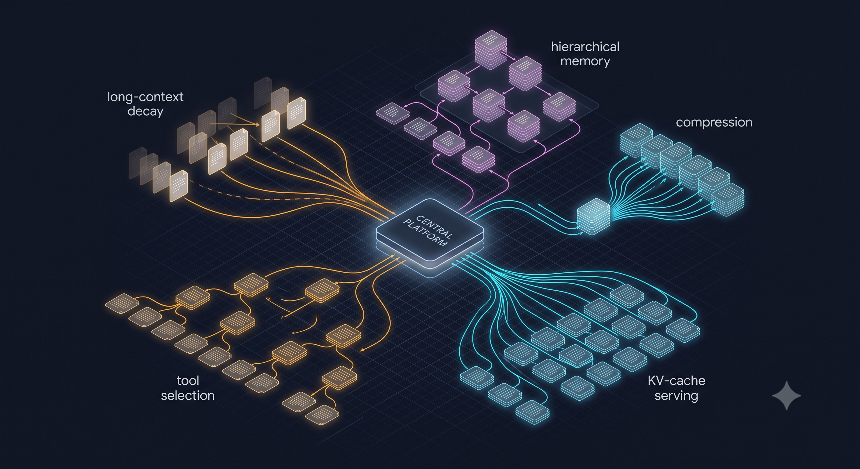
Why long context degrades (motivates all curation). Lost in the Middle (Liu et al., 2023, arXiv:2307.03172) — U-shaped positional attention. RULER (Hsieh et al., 2024) — effective context ≪ advertised. NoLiMa (Modarressi et al., ICML 2025, arXiv:2502.05167) — remove lexical overlap and 11/13 models fall below 50% of baseline by 32K; defines effective length as ≥85%-of-base. Chroma context-rot study (2025) — all 18 models degrade with length; recency bias means ordering inside the window matters.
Hierarchical memory (Strategy 4). MemGPT (Packer et al., 2023, arXiv:2310.08560) → Letta. Mem0 (Chhikara et al., ECAI 2025, arXiv:2504.19413) — production numbers: 91% lower p95 latency, ~90% fewer tokens, +26% accuracy vs full-context. A-Mem (Xu et al., 2025) — evolving Zettelkasten memory notes. Benchmarks: LoCoMo (Maharana et al., 2024), LongMemEval (Wu et al., ICLR 2025, ~30-pt oracle gap), BEAM (1M/10M scale). Recurrent Memory Transformer (Bulatov et al., 2022, arXiv:2207.06881) — the learned-memory-token end-state these systems approximate.
Prompt / context compression (Strategy 6). LLMLingua + LongLLMLingua (Jiang et al., 2023, arXiv:2310.05736, 2310.06839) — ~20× at under 2% loss. RECOMP (Xu et al., 2023, arXiv:2310.04408) — trained RAG compressor beating zero-shot summarization.
Tool selection at scale (Strategies 2, 8). RAG-MCP (Gan & Sun, 2025, arXiv:2505.03275) — retrieval over MCP index, >50% tokens, 3× accuracy, stress-tested to 11,100 tools. Gorilla (Patil et al., 2023, arXiv:2305.15334) and Toolformer (Schick et al., 2023, arXiv:2302.04761) — the tool-use foundations. Thompson-sampling-for-tool-use — active NeurIPS/ICML 2024–2026 workshop thread; cite current best at publish time.
Agent reasoning / external memory patterns. LATS (arXiv:2310.04406), Reflexion (Shinn et al., 2023, arXiv:2303.11366), Chain-of-Note (arXiv:2311.09210) — self-critique and external-note patterns that feed working-state and reward design.
Serving-layer KV cache (Strategies 1, 7 when self-hosting — Section 07). PagedAttention / vLLM (Kwon et al., SOSP 2023, arXiv:2309.06180). RadixAttention / SGLang (Zheng et al., NeurIPS 2024, arXiv:2312.07104). KVFlow (arXiv:2507.07400, 2025) — multi-agent prefix-cache scheduling, 1.83× over SGLang. Mooncake (Qin et al., 2024) — KVCache-centric disaggregated serving. LMCache (arXiv:2510.09665), TokenCake (arXiv:2510.18586), CacheBlend (arXiv:2405.16444), RAGCache (arXiv:2404.12457), TurboRAG (arXiv:2410.07590) — cross-request and RAG-specific KV reuse.
Standards. Model Context Protocol (Anthropic). OpenTelemetry GenAI semantic conventions (token/latency telemetry).
11 — The build order (do exactly this)
Deviating usually costs more than following it. Weeks are for one senior engineer atop a working agent loop.
| Step | Strategy / task | Weeks | Prereq |
|---|---|---|---|
| 0a | Per-turn token accounting (OTel GenAI conventions) | 1 | — |
| 0b | Ground-truth reward signal | 1 | — |
| 0c | Storage tiers stood up (Redis / log sink / vector DB) | 1 | — |
| 1 | Prompt caching on stable prefixes (4 boundaries, explicit TTL) | 1 | 0a |
| 2 | Tool retrieval: semantic top-k + describe_tool | 2 | 0a, 1 |
| 3 | Tiered memory (log + typed working state + cross-session) | 2 | 0a, 0c |
| 4 | Anchored compaction with pinned invariants (or server-side compaction) | 1 | 3 |
| 5 | Golden-fact verification on summaries | 2 | 4 |
| 6 | Subagent isolation per MCP with tool scoping | 3 | 2, 3 |
| 7 | Bandit scoring (Beta-Bernoulli + Thompson) | 3 | 0b, 2 |
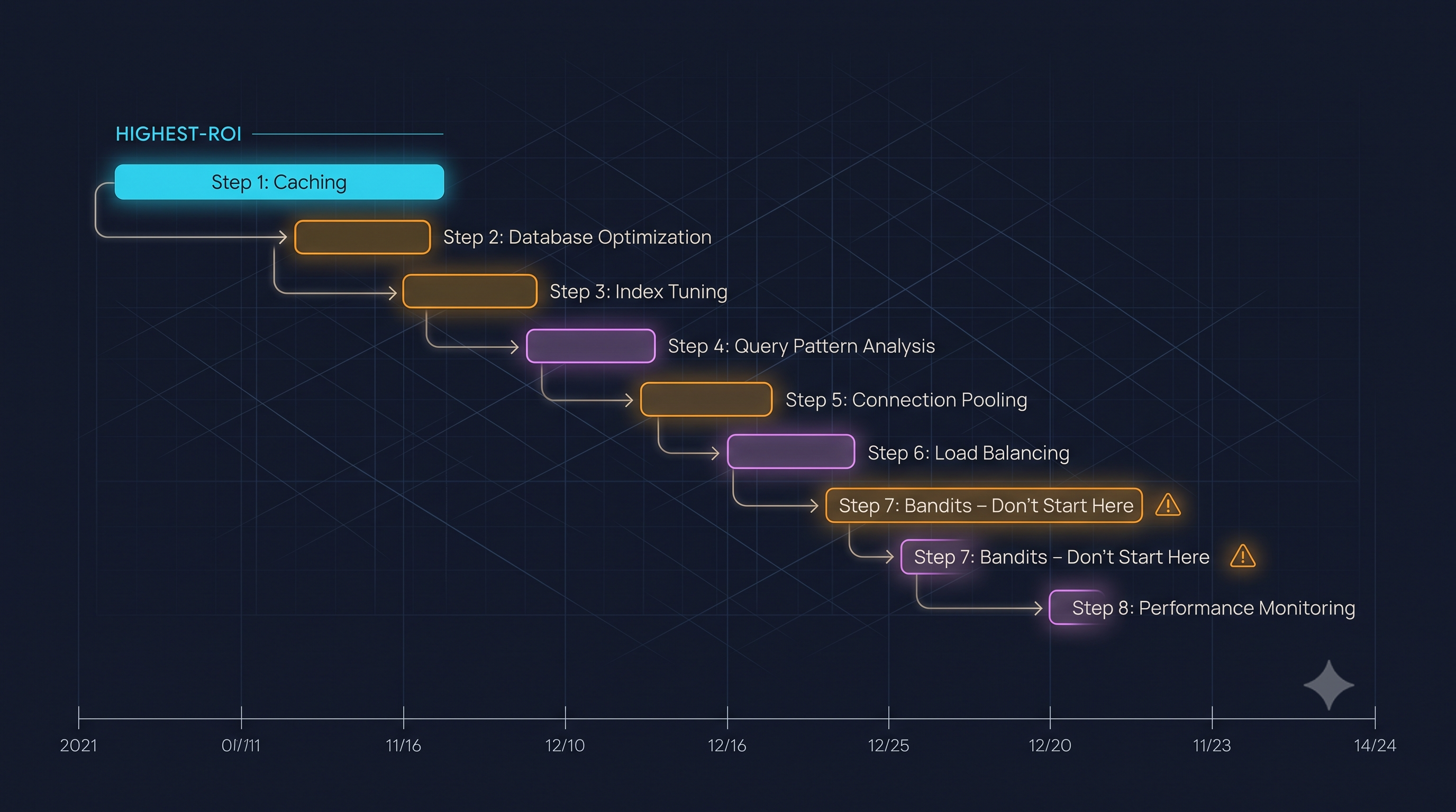
Total ≈ 17 weeks — roughly one quarter — to a fully optimized stack. Add a latency budget (Section 05) as a cross-cutting requirement on every step, and revisit Section 07 as a fork if you offer self-hosted models.
The common failure mode is starting at Step 7 because bandits are the most intellectually interesting. They are the least valuable if the earlier steps aren’t done — a self-tuning selector atop uncached prefixes and uncompacted history is a race engine bolted to a car with no wheels. Prompt caching alone — two days — delivers 60–80% of the total available savings and a latency win. Do the boring, high-leverage things first; the interesting things pay off only once the boring ones are in place.
12 — The 2027+ direction
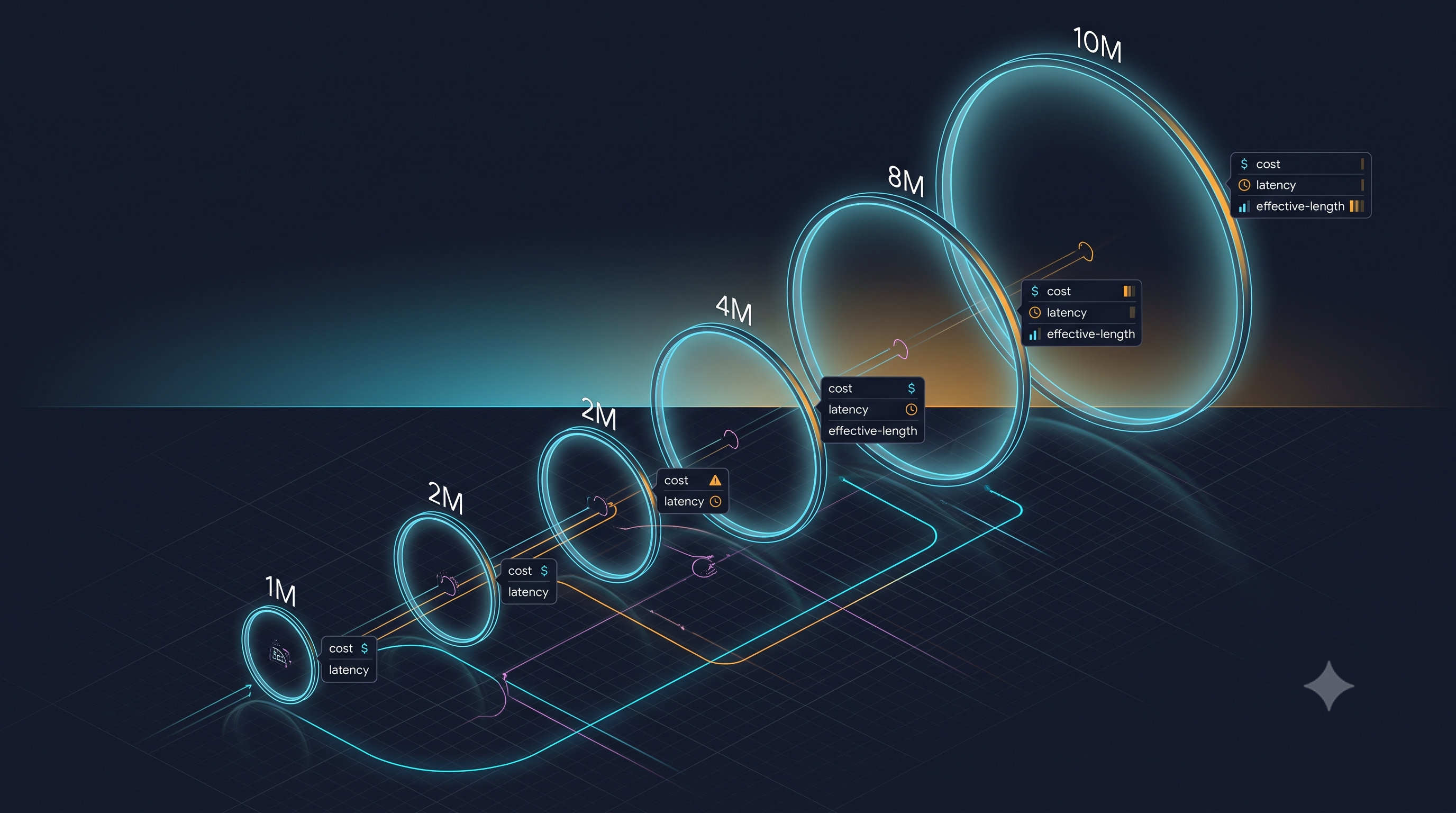
Long-context models blunt raw-window pain: 1M windows at standard pricing (Sonnet 4.6, Opus 4.x), Llama 4 Scout’s 10M open-weight window, DeepSeek/Qwen extending context, and attention-efficiency work making those windows practically usable. Thirteen-plus hosted models now ship ≥1M windows, and filling one costs between $0.14 and $10.00 — a 71× spread. It is tempting to conclude the problem dissolves.
It does not, for three durable reasons. Cost is permanent: even a 10M-context model bills per input token (or per GPU-second), so context efficiency stays a P&L discipline forever; only the pain threshold moves. Effective context is permanent: NoLiMa and context rot are properties of attention, not of window size — a bigger window with an unchanged effective length is a longer rope to hang quality with, which is why every strategy here survives the window increase. Latency is permanent: prefill is quadratic regardless of the limit, so shrinking the prefix will always buy TTFT.
The likely evolution is that these strategies stop being per-team engineering and become platform primitives. Server-side compaction and context editing already shipped as API features in 2026; expect bandit-based tool selection, typed working state, and memory tiers to follow — bundled by observability and agent-infra vendors (LangSmith, Phoenix, Helicone, Letta, Mem0) and standardized onto OpenTelemetry GenAI telemetry so cost and latency are portable across providers and across the hosted/self-hosted line.
References
- Liu, N. F., Lin, K., Hewitt, J., Paranjape, A., Hopkins, M., Luck, F., & Manning, C. D. (2023). Lost in the Middle: How Language Models Use Long Contexts. arXiv:2307.03172.
- Modarressi, A., Farahani, M., Rezaei, S., & Pilehvar, M. T. (2025). NoLiMa: Non-Linear Memory Attention Benchmark. ICML 2025. arXiv:2502.05167.
- Packer, C., Wooders, S., Lin, K., Fang, V., Patil, S. G., Stoica, I., & Gonzalez, J. E. (2023). MemGPT: Towards LLMs as Operating Systems. arXiv:2310.08560.
- Chhikara, P., et al. (2025). Mem0: The Memory Layer for Personalized AI. ECAI 2025. arXiv:2504.19413.
- Gan, Y., & Sun, J. (2025). RAG-MCP: Mitigating Prompt Bloat in LLM Tool Selection via Retrieval-Augmented Generation. arXiv:2505.03275.
- Jiang, H., et al. (2023). LLMLingua: Compressing Prompts for Accelerated Inference of Large Language Models. arXiv:2310.05736.
- Jiang, H., et al. (2023). LongLLMLingua: Accelerating and Enhancing LLMs in Long Context Scenarios via Prompt Compression. arXiv:2310.06839.
- Xu, F. F., et al. (2023). RECOMP: Improving Retrieval-Augmented LMs with Context Compression and Selective Augmentation. arXiv:2310.04408.
- Kwon, W., et al. (2023). Efficient Memory Management for Large Language Model Serving with PagedAttention. SOSP 2023. arXiv:2309.06180.
- Zheng, L., et al. (2024). SGLang: Efficient Execution of Structured Language Model Programs. NeurIPS 2024. arXiv:2312.07104.
- KVFlow Team (2025). KVFlow: Workflow-Aware KV Cache Scheduling for Multi-Agent LLM Workloads. arXiv:2507.07400.
- Bulatov, A., Kuratov, Y., & Burtsev, M. (2022). Recurrent Memory Transformer. arXiv:2207.06881.
- Shinn, N., Cassano, F., Labash, B., Gopalan, A., Narasimhan, K., & Yao, S. (2023). Reflexion: Language Agents with Verbal Reinforcement Learning. arXiv:2303.11366.
- Patil, S. G., Zhang, T., Wang, X., & Gonzalez, J. E. (2023). Gorilla: Large Language Model Connected with Massive APIs. arXiv:2305.15334.
- Schick, T., et al. (2023). Toolformer: Language Models Can Teach Themselves to Use Tools. arXiv:2302.04761.
- Zhou, A., et al. (2023). Language Agent Tree Search Unifies Reasoning, Acting, and Planning in Language Models. arXiv:2310.04406.
- Wang, Z., et al. (2023). Chain-of-Note: Enhancing Robustness in Retrieval-Augmented Language Models. arXiv:2311.09210.
- Yao, Z., et al. (2024). CacheBlend: Fast Large Language Model Serving for RAG with Cached Knowledge Fusion. arXiv:2405.16444.
- Jin, C., et al. (2024). RAGCache: Efficient Knowledge Caching for Retrieval-Augmented Generation. arXiv:2404.12457.
- Liu, Z., et al. (2025). LMCache: Enabling Efficient LLM Serving via KV Cache Reuse. arXiv:2510.09665.
- TokenCake Team (2025). TokenCake: Maximizing GPU Utilization in Multi-Agent LLM Serving. arXiv:2510.18586.
- Lyu, J., et al. (2024). TurboRAG: Accelerating Retrieval-Augmented Generation with Precomputed KV Caches for Chunked Text. arXiv:2410.07590.
BibTeX
@article{fp4-2607001,
  title   = {Context Window Management for Multi-Agentic Platforms},
  author  = {fp4 editorial desk},
  year    = {2026},
  url     = {https://fp4.dev/algorithm/context-window-multi-agent/},
  journal = {fp4}
}